提示:文章写完后,目录可以自动生成,如何生成可参考右边的帮助文档
前言
空域滤波增强
- 卷积原理
- 多维连续卷积
- 线性平滑滤波
- 领域平均法、选择平均法、Wiener滤波
- 非线性平滑滤波
- 中值滤波
- 线性锐化滤波
- Laplacian算子
- 非线性锐化滤波
- Prewitt算子
- Sobel算子
- Log算子
Matlab学习7-图像处理之线性平滑滤波
领域平均法、选择平均法、Wiener滤波
一、选择平均法滤波去噪
效果
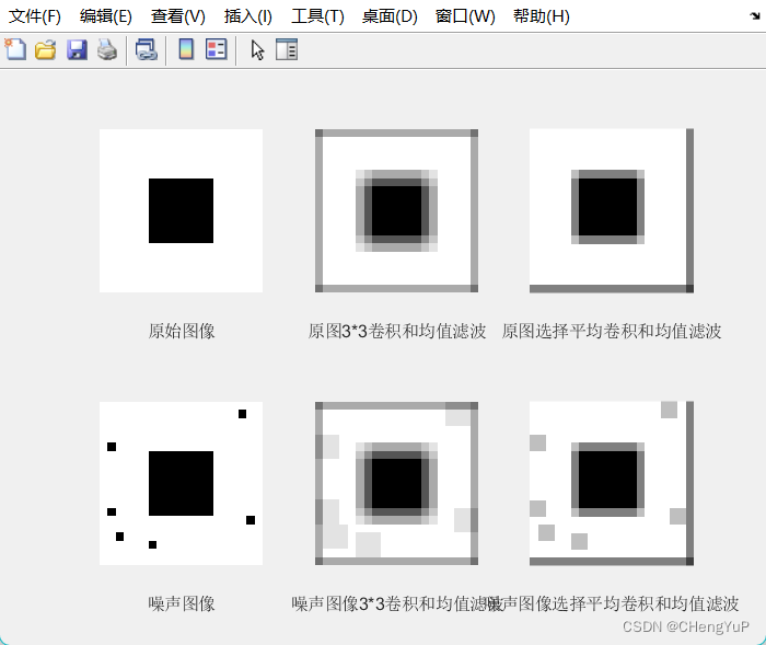
代码
% 选择平均法滤波去噪
img =imread("img/test.bmp");
subplot(2,3,1);imshow(img),xlabel("原始图像");

% 均值滤波
K1=filter2(fspecial("average",3),img);
subplot(2,3,2);imshow(uint8(K1)),xlabel("原图3*3卷积和均值滤波");

%卷积和 或模板
mask=[  0 0 0
        0 1 1
        0 1 1];
mask=1/4*mask;
K2=filter2(mask,img);
subplot(2,3,3);imshow(uint8(K2)),xlabel("原图选择平均卷积和均值滤波");

ju=imnoise(img,"salt & pepper",0.04);
subplot(2,3,4);imshow(ju),xlabel("噪声图像");

% 均值滤波
K3=filter2(fspecial("average",3),ju);
subplot(2,3,5);imshow(uint8(K3)),xlabel("噪声图像3*3卷积和均值滤波");
%卷积和 或模板
mask=[  0 0 0
        0 1 1
        0 1 1];
mask=1/4*mask;
K4=filter2(mask,ju);
subplot(2,3,6);imshow(uint8(K4)),xlabel("噪声图像选择平均卷积和均值滤波");
二、领域平均法去噪
效果
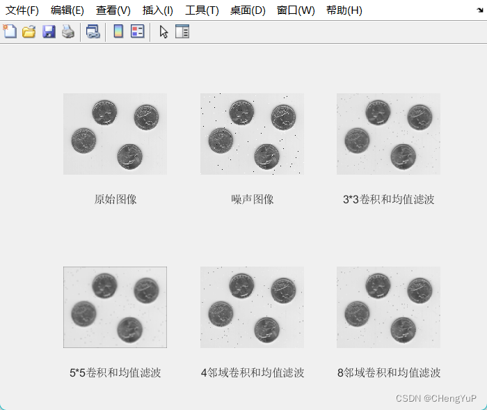
代码
%领域平均法去噪
img =imread("img/eight.tif");
subplot(2,3,1);imshow(img),xlabel("原始图像");

ju=imnoise(img,"salt & pepper",0.004);
subplot(2,3,2);imshow(ju),xlabel("噪声图像");
% 均值滤波
K1=filter2(fspecial("average",3),ju);
subplot(2,3,3);imshow(uint8(K1)),xlabel("3*3卷积和均值滤波");

K2=filter2(fspecial("average",5),ju);
subplot(2,3,4);imshow(uint8(K2)),xlabel("5*5卷积和均值滤波");

%卷积和 或模板
mask4=[ 0 1 0
        1 0 1
        0 1 0];
mask4=1/4*mask4;
K3=filter2(mask4,ju);
subplot(2,3,5);imshow(uint8(K3)),xlabel("4邻域卷积和均值滤波");


mask8=[ 1 1 1
        1 0 1
        1 1 1];
mask8=1/8*mask8;
K4=filter2(mask8,ju);
subplot(2,3,6);imshow(uint8(K4)),xlabel("8邻域卷积和均值滤波");
三、Wiener滤波
效果
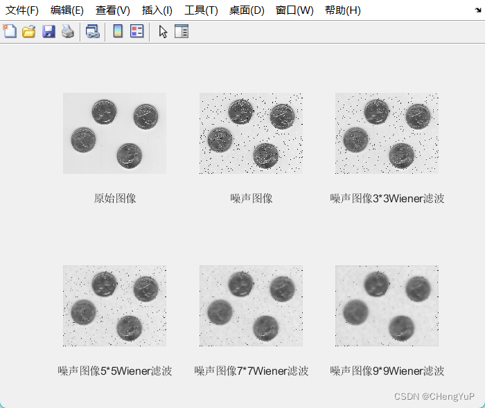
代码
% Wiener滤波
img =imread("img/eight.tif");
subplot(2,3,1);imshow(img),xlabel("原始图像");
ju=imnoise(img,"salt & pepper",0.04);
subplot(2,3,2);imshow(ju),xlabel("噪声图像");

K1=wiener2(ju,[3,3]);
subplot(2,3,3);imshow(K1),xlabel("噪声图像3*3Wiener滤波");
K2=wiener2(ju,[5,5]);
subplot(2,3,4);imshow(K2),xlabel("噪声图像5*5Wiener滤波");
K3=wiener2(ju,[7,7]);
subplot(2,3,5);imshow(K3),xlabel("噪声图像7*7Wiener滤波");
K4=wiener2(ju,[9,9]);
subplot(2,3,6);imshow(K4),xlabel("噪声图像9*9Wiener滤波");
四、线性平滑滤波
代码
%线性平滑滤波
Fxy=[0 20 40 70
    80 100 120 150
    160 180 200 230];
uint8Fxy=uint8(Fxy);
subplot(2,2,1),imshow(uint8Fxy),xlabel("原始图像");
subplot(2,2,2),imhist(uint8Fxy),axis([0,255,0,1]),xlabel("原始图像的直方图","position",[120,-0.23]);

%平滑操作,作用模糊,去噪
Gxy=filter2(fspecial("average",3),uint8Fxy);
uint8Gxy=uint8(Gxy);
subplot(2,2,3),imshow(uint8Gxy),xlabel("均值滤波后的图像");
subplot(2,2,4),imhist(uint8Gxy),axis([0,255,0,1]),xlabel("滤波后图像的直方图","position",[120,-0.23]);
点击获取源码
https://gitee.com/CYFreud/matlab/tree/master/image_processing/demo7_220418