1 为什么学习变换 Why study transformation

1.1 模型变换 Modeling

场景展示——描述摄像机的位置移动
机器人跳舞——物体的旋转
皮克斯开场动画台灯压扁字母I——物体的缩放

1.2 视图变换 Viewing

光栅化成像中涉及大量的视图变换

2 二维变换 2D Transformations

3B1B线代的本质（可视化理解线性变换）：https://www.bilibili.com/video/BV1ns41167b9?spm_id_from=333.999.0.0

2.1 缩放变换矩阵 Scale Matrix

不锁定比例的 Non-Uniform

$\begin{pmatrix} { } { x ^ { \prime } } \\ { y ^ { \prime } } \end{pmatrix} = \begin{pmatrix} { } { s _ { x } } & { 0 } \\ { 0 } & { s _ { y } } \end{pmatrix} \begin{pmatrix} { } { x } \\ { y } \end{pmatrix}$

2.2 对称变换矩阵 Reflection Matrix

水平翻转 Horizontal reflection：

$\begin{pmatrix} { } { x ^ { \prime } } \\ { y ^ { \prime } } \end{pmatrix} = \begin{pmatrix} { } { - 1 } & { 0 } \\ { 0 } & { 1 } \end{pmatrix} \begin{pmatrix} { } { x } \\ { y } \end{pmatrix}$

2.3 切变变换矩阵 Shear Matrix

水平方向位移在y=0处是0，在y=1处是a，竖直方向位移总是0

$\begin{pmatrix} { } { x ^ { \prime } } \\ { y ^ { \prime } } \end{pmatrix} = \begin{pmatrix} { } { 1 } & { a } \\ { 0 } & { 1 } \end{pmatrix} \begin{pmatrix} { } { x } \\ { y } \end{pmatrix}$

2.4 旋转变换矩阵(默认绕原点、逆时针方向) Rotation Matrix

旋转的角度为θ

$\theta } = \begin{pmatrix} { } { \cos \theta } & { -\sin \theta } \\ { \sin \theta } & { \cos \theta } \end{pmatrix}$

2.5 线性变换 Linear Transforms

使用相同维度的矩阵相乘，形式为坐标与矩阵相乘得到新的坐标
$\begin{pmatrix} { } { x ^ { \prime } } \\ { y ^ { \prime } } \end{pmatrix} = \begin{pmatrix} { } { a } & { b } \\ { c } & { d } \end{pmatrix} \begin{pmatrix} { } { x } \\ { y } \end{pmatrix}$

3 齐次坐标 Homogeneous Coordinates

3.1 为什么学习齐次坐标 Why homogeneous coordinates

平移变换不是线性变换，无法直接用矩阵形式表示

$\begin{pmatrix} { } { x ^ { \prime } } \\ { y ^ { \prime } } \end{pmatrix} = \begin{pmatrix} { } { a } & { b } \\ { c } & { d } \end{pmatrix} \begin{pmatrix} { } { x } \\ { y } \end{pmatrix} + \begin{pmatrix} { } { t _ { x } } \\ { t y } \end{pmatrix}$

我们不想把平移当作一个特殊的变换 But we don’t want translation to be a special case
是否有一种统一的方式能够表示所有变换，它的代价怎么样？ Is there a unified way to represent all transformations? (and what’s the cost?)

3.2 通过齐次坐标解决问题 Solution: Homogenous Coordinates

3.2.1 添加第三个坐标 Add a third coordinate (w-coordinate)

$\rm{2D\,point}=(x,y,1)^T,\quad\rm{2D\,vector}=(x,y,0)^T$

3.2.2 平移的矩阵表示 Matrix representation of translations

$\begin{pmatrix} { } { x ^ { \prime } } \\ { y ^ { \prime } } \\ { w ^ { \prime } } \end{pmatrix} = \begin{pmatrix} { } { 1 } & { 0 } & { t_x } \\ { 0 } & { 1 } & { t_y } \\ { 0 } & { 0 } & { 1 } \end{pmatrix}\cdot\begin{pmatrix} { } { x } \\ { y } \\ { 1 } \end{pmatrix} = \begin{pmatrix} { } { x + t_x } \\ { y + t_y } \\ { 1 } \end{pmatrix}$

3.2.3 如果平移的是一个向量？ What if you translate a vector?

向量具有平移不变性，经过平移变换后还是原向量
$\begin{pmatrix} { } { x ^ { \prime } } \\ { y ^ { \prime } } \\ { w ^ { \prime } } \end{pmatrix} = \begin{pmatrix} { } { 1 } & { 0 } & { t_x } \\ { 0 } & { 1 } & { t_y } \\ { 0 } & { 0 } & { 1 } \end{pmatrix}\cdot\begin{pmatrix} { } { x } \\ { y } \\ { 0 } \end{pmatrix} = \begin{pmatrix} { } { x } \\ { y } \\ { 0 } \end{pmatrix}$

3.2.4 齐次坐标的妙处

如果w-coordinate的结果是1或0则为有效操作，这样既能让平移变换形式统一，也保留了向量和点加减运算的可操作性
使用齐次坐标时，(x, y, w)表示平面内一点(x/w, y/w, 1), w≠0
- vector + vector = vector 0+0=0
- point – point = vector 1-1=0
- point + vector = point 1+0=1
- point + point = ??

point+point得到的结果为两个点连线的中点（将w-coordinate化为1）

3.2.5 仿射变换 Affine Transformations

仿射变换 = 线性变换 + 平移变换 Affine map = linear map + translation
$\begin{pmatrix} { } { x ^ { \prime } } \\ { y ^ { \prime } } \end{pmatrix} = \begin{pmatrix} { } { a } & { b } \\ { c } & { d } \end{pmatrix} \cdot \begin{pmatrix} { } { x } \\ { y } \end{pmatrix} + \begin{pmatrix} { } { t_x } \\ { t_y } \end{pmatrix}$
使用齐次坐标 Using homogenous coordinates:
$\rm{Affine\;Transformations：}\begin{pmatrix} { } { x ^ { \prime } } \\ { y ^ { \prime } } \\ { 1 } \end{pmatrix} = \begin{pmatrix} { } { a } & { b } & { t _ { x } } \\ { c } & { d } & { t _ { y } } \\ { 0 } & { 0 } & { 1 } \end{pmatrix} \cdot \begin{pmatrix} { } { x } \\ { y }\\{1} \end{pmatrix}$

3.2.6 使用齐次坐标的2D变换 2D Transformations

$\rm{Scale：}S (s _ { x , } s _ { y } ) = \begin{pmatrix} {} { s _ { x } } & { 0 } & { 0 } \\ { 0 } & { s _ { y } } & { 0 } \\ { 0 } & { 0 } & { 1 } \end{pmatrix}$

$\rm{Rotation：}R ( \alpha ) = \begin{pmatrix} {} { \cos \alpha } & { - \sin \alpha } & { 0 } \\ { \sin \alpha } & { \cos \alpha } & { 0 } \\ { 0 } & { 0 } & { 1 } \end{pmatrix}$

$\rm{Translation：}T ( t _ { x , } t _ { y } ) = \begin{pmatrix} { } { 1 } & { 0 } & { t x } \\ { 0 } & { 1 } & { t _ { y } } \\ { 0 } & { 0 } & { 1 } \end{pmatrix}$

齐次坐标的代价是引入了额外的数字参与计算

4 逆变换 Inverse Transform

$M^{-1}$ 既是M矩阵的逆，也是矩阵几何意义上的逆

5 组合变换 Composite Transform

5.1 变换的顺序会影响结果！ Transform Ordering Matters!

先平移后旋转与先旋转后平移
从矩阵的运算来看，矩阵的乘法不满足交换律 Matrix multiplication is not commutative
$R45 \cdot T _ { ( 1 , 0 ) } \neq T _ { ( 1 , 0 ) } \cdot R _ { 45 }$
注意矩阵的运算顺序是从右到左的 Note that matrices are applied right to left
$\cdot R _ { 45 } \begin{pmatrix} { } { x } \\ { y } \\ { 1 } \end{pmatrix} = \begin{pmatrix} {} { 1 } & { 0 } & { 1 } \\ { 0 } & { 1 }&{0} \\ { 0 } & { 0 } & { 1 } \end{pmatrix}\begin{pmatrix} { } { \cos 45 ^ { \circ } } & { - \sin 45 ^ { \circ } } & { 0 } \\ { \sin 45 ^ { \circ } } & { \cos 45 ^ { \circ } } & { 0 } \\ { 0 } & { 0 } & { 1 } \end{pmatrix} \begin{pmatrix} { } { x } \\ { y } \\ { 1 } \end{pmatrix}$

5.2 组合变换 Composite Transform

对于仿射变换序列A₁, A₂, A₃, …可以先使用结合律得到一个表示组合变换的单个矩阵，这一点对性能消耗十分重要！
$An \cdots A _ { 2 } ( A _ { 1 } ( X ) ) ) =\underbrace{ A _ { n } \cdots A _ { 2 } \cdot A _ { 1 } }_{\rm{Pre-multiply}}\cdot \begin{pmatrix} {} { x } \\ { y } \\ { 1 } \end{pmatrix}$

6 分解复杂的变换 Decomposing Complex Transforms

如何以任意一点c为圆心旋转 How to rotate around a given point c?
- 先把旋转中心点平移到原点 Translate center to origin
- 旋转 Rotate
- 平移到原位置 Translate back

7 三维变换 3D Transformations

7.1 使用齐次坐标描述三维空间中的点和向量

再一次使用齐次坐标 Use homogeneous coordinates again:
$\rm{3D\,point}=(x,y,z,1)^T,\quad\rm{3D\,vector}=(x,y,z,0)^T$
使用齐次坐标时，(x, y, z, w)表示三维空间内一点(x/w, y/w, z/w), w≠0
使用4×4矩阵来表示仿射变换 Use 4×4 matrices for affine transformation
$\begin{pmatrix} {} { x ^ { \prime } } \\ { y ^ { \prime } } \\ { z ^ { \prime } } \\ { 1 } \end{pmatrix} =\begin{pmatrix} { } { a } & { b } & { c } & { t _ { x } } \\ { d } & { e } & { f } & { t _ { y } } \\ { g } & { h } & { i } & { t _ { z } } \\ { 0 } & { 0 } & { 0 } & { 1 } \end{pmatrix}\cdot\begin{pmatrix} { } { x } \\ { y } \\ { z } \\ { 1 } \end{pmatrix}$
仿射变换的顺序是先进行线性变换，再平移

7.2 三维空间中的缩放与平移 Scale and Translation

缩放 Scale
$\begin{pmatrix} {} { s _ { x } } & { 0 } & { 0 } & { 0 } \\ { 0 } & { s _ { y } } & { 0 } & { 0 } \\ { 0 } & { 0 } & { s_z } & { 0 } \\ { 0 } & { 0 } & { 0 } & { 1 }\end{pmatrix}$
平移 Translation
$\begin{pmatrix} { } { 1 } & { 0 } & { 0 } & { t _ { x } } \\ { 0 } & { 1 } & { 0 } & { t _ { y } } \\ { 0 } & { 0 } & { 1 } & { t _ { z } } \\ { 0 } & { 0 } & { 0 } & { 1}\end{pmatrix}$

7.3 三维空间中的旋转 3D Rotations

7.3.1 沿x，y，z轴旋转 Rotation around x-, y-, or z-axis

在这里插入图片描述

$\alpha ) = \begin{pmatrix} { } { 1 } & { 0 } & { 0 } & { 0 } \\ { 0 } & { \cos \alpha } & { - \sin \alpha } & { 0 } \\ { 0 } & { \sin \alpha } & { \cos \alpha } & { 0 } \\ { 0 } & { 0 } & { 0 } & { 1 } \end{pmatrix}$
$\alpha ) = \begin{pmatrix} {} { \cos \alpha } & { 0 } & { \sin \alpha } & { 0 } \\ { 0 } & { 1 } & { 0 } & { 0 } \\ { - \sin \alpha } & { 0 } & { \cos \alpha } & { 0 } \\ { 0 } & { 0 } & { 0 } & { 1 } \end{pmatrix}$
$\alpha ) = \begin{pmatrix} { } { \cos \alpha } & { - \sin \alpha } & { 0 } & { 0 } \\ { \sin \alpha } & { \cos \alpha } & { 0 } & { 0 } \\ { 0 } & { 0 } & { 1 } & { 0 } \\ { 0 } & { 0 } & { 1 } & { 0 } \end{pmatrix}$

注意：沿y轴旋转时矩阵稍有不同（z叉乘x得到y轴，而不是x叉乘z）
弹幕解释：xyz，yzx，zxy，这三个没有本质区别，懂了这个，前面迎刃而解

7.3.2 任意一个旋转能看作几个绕轴旋转的组合 Compose any 3D rotation from Rx, Ry, Rz

三个一组的描述物体旋转的参量叫欧拉角 Euler angles
在飞行模拟器中一般有滚转、俯仰、偏航 Often used in flight simulators: roll, pitch, yaw
罗德里格旋转公式 Rodrigues’ Rotation Formula
$\rm{绕n轴旋转\alpha角度：} ( n , \alpha ) = \cos ( \alpha ) I + ( 1 - \cos ( \alpha ) ) n n ^ { T } +\sin ( \alpha ) \underbrace{\begin{pmatrix} { } { 0 } & { - n _ { z } } & { n _ { y } } \\ { n _ { z } } & { 0 } & { - n _ { x } } \\ { - n _ { y } } & { n _ { x } } & { 0 } \end{pmatrix}}_{\rm{N}}$
如果要沿任意轴旋转，和二维类似，需要先把旋转的起点移到轴上，然后旋转，最后再移回原位
四元数(Quaternion)的引入主要是为了解决旋转角度间的插值问题，本课暂不涉及

8 观测变换 Viewing transformation

8.1 视图变换 View/Camera transformation

8.1.1 什么是视图变换 What is view transformation?

想象一下如何拍一张照片 Think about how to take a photo
1. 找个地方安排人（模型变换）Find a good place and arrange people (model transformation)
2. 找个“角度”放相机（视图变换）Find a good “angle” to put the camera (view transformation)
3. 茄子！（投影变换）Cheese! (projection transformation)

8.1.2 如何确定视图变换 How to perform view transformation?

定义一个相机
- 确定位置 Position $\vec{e}$
- 确定看向的方向 Look-at / gaze direction $\hat{g}$
- 确定向上方向（来确定相机左右倾斜方向）Up direction $\hat{t}$

8.1.3 标准位置 Key observation

相机和物体的相对位置不变，则画面也不变 If the camera and all objects move together, the “photo” will be the same
我们通常将相机的位置移动到原点、向上方向为Y轴方向、看向-Z轴方向，物体与相机同时变换we always transform the camera to the origin, up at Y, look at -Z, and transform the objects along with the camera
通过矩阵 $M_{view}$ 来对相机进行变换 Transform the camera by $M_{view}$
$M_{view}=R_{view}T_{view}$
1. 平移到原点 Translate e to origin
  $\begin{pmatrix} { } { 1 } & { 0 } & { 0 } & { - x _ { c } } \\ { 0 } & { 1 } & { 0 } & { - y _ { c } } \\ { 0 } & { 0 } & { 1 } & { - z_c } \\ { 0 } & { 0 } & { 0 } & { 1 } \end{pmatrix}$
2. 将g旋转到-Z，t旋转到Y，(g×t)旋转到X Rotate g to -Z, t to Y, (g x t) To X
  $R^{-1}_{view}=\begin{pmatrix} {} { x _ { \hat{g} \times \hat{t}} } & { x _ { t } } & { x _ { -g } } & { 0 } \\ { y _ { \hat{g} \times \hat{t}} } & { y _ { t } } & { y _ { - g } } & { 0 } \\ { z _ {\hat{g} \times \hat{t}}} & { z _ { t } } & { z _ { - g } } & { 0 } \\ { 0 } & { 0}&{0}&{1}\end{pmatrix}\implies R_{view}=\begin{pmatrix} {} { x _ { \hat{g} \times \hat{t}} } & { y _ { \hat{g} \times \hat{t}} } & { z _ { \hat{g} \times \hat{t}} } & { 0 } \\ { x _ { t } } & { y _ { t } } & { z _ { t } } & { 0 } \\ { x _ { - g } } & { y _ { - g } } & { z _ { - g } } & { 0 } \\ { 0 } & { 0 }&{ 0 }&{ 1 }\end{pmatrix}$

旋转矩阵是正交矩阵(Orthogonal Matrix)，这里因其逆矩阵比较好写出来，所以利用了正交矩阵的逆等于其转置的性质求出了旋转矩阵

8.2 投影变换 Projection transformation

8.2.1正交投影与透视投影 Perspective projection vs. orthographic projection

人眼更接近透视投影，正交投影常用于工业制图
“近大远小““一叶障目”“道理我都懂但是鸽子为什么这么大”都指的是透视投影

在这里插入图片描述

8.2.2 正交投影 Othographic projection

简单的理解 A simple way of understanding

相机在原点，朝向-Z方向，上指Y方向 Camera located at origin, looking at -Z, up at Y
去掉Z轴坐标 Drop Z coordinate
将得到的矩形平移并缩放到 $1, 1]^2$ Translate and scale the resulting rectangle to $1, 1]^2$

正式的理解 In general

我们希望将一个立方体空间 $[l, r] \times [b, t] \times [f, n]$ 映射成一个标准的正方体 $1, 1]^3$ We want to map a cuboid $[l, r] \times [b, t] \times [f, n]$ to the “canonical cube $1, 1]^3$
在变换时先平移(中心移到原点)，再缩放(长宽高变为2) Translate (center to origin) first, then scale (length/width/height to 2)
$M_{ortho}=\begin{pmatrix} { } { \frac { 2 } { r - l } } & { 0 } & { 0 } & { 0 } \\ { 0 } & { \frac { 2 } { t - b } } & { 0 } & { 0 } \\ { 0 } & { 0 } & { \frac { 2 } { n - f } } & { 0 } \\ { 0 } & { 0 } & { 0 } & { 1 } \end{pmatrix}\begin{pmatrix} {} { 1 } & { 0 } & { 0 } & { - \frac { r + l } { 2 } } \\ { 0 } & { 1 } & { 0 } & { - \frac { t + b } { 2 } } \\ { 0 } & { 0 } & { 1 } & { - \frac { n + f } { 2 } } \\ { 0 } & { 0 } & { 0 } & { 1 } \end{pmatrix}$
注意事项
- 相机看向-Z方向时近的坐标会大于远的坐标 Looking at / along -Z is making near and far not intuitive (n > f)
- 这也是为什么OpenGL在这一步使用左手坐标系 that’s why OpenGL (a Graphics API) uses left hand coords

8.2.3 透视投影 Perspective projection

怎样做透视投影？

首先将截头体“挤压”成一个长方体 First “squish” the frustum into a cuboid (n -> n, f -> f)( $M_{persp\to ortho}$ )
做正交投影 Do orthographic projection ( $M_{ortho}$ , already known!)

“挤压”变换的矩阵推导过程

由相似三角形可得到坐标变换前后的关系 Find the relationship between transformed points (x’, y’, z’) and the original points (x, y, z)

$y\prime=\frac{n}{z}y\rm{，}x\prime=\frac{n}{z}x$
2. 此时利用齐次坐标可以写出含有一个未知数的变换后的坐标 In homogeneous coordinates
$\begin{pmatrix} { } { x } \\ { y } \\ { z } \\ { 1 } \end{pmatrix} \Rightarrow \begin{pmatrix} { } { n x / z } \\ { n y / z } \\ { un k n o wn} \\ { 1 } \end{pmatrix} = = \begin{pmatrix} { } { n y } \\ { n y} \\ { still\;unk n o w n }\\{z} \end{pmatrix}$
3. 所以“挤压”变换的矩阵有如下关系 So the “squish” (persp to ortho) projection does this
$M^{(4×4)}_{persp\to ortho}\begin{pmatrix} { } { x } \\ { y } \\ { z } \\ { 1 } \end{pmatrix} = \begin{pmatrix} { } { n x } \\ { n y } \\ {unknown} \\{ z } \end{pmatrix}$
4. 以上信息我们已经可以填出一部分 $M_{persp\to ortho}$ Already good enough to figure out part of $M_{persp\to ortho}$ （接下来只用找出该矩阵第三行上的数到底是多少即可）
$M_{persp\to ortho}=\begin{pmatrix} { } { n } & { 0 } & { 0 } & { 0 } \\ { 0 } & { n } & { 0 } & { 0 } \\ { ? } & { ? } & { ? } & { ? } \\ { 0 } & { 0 } & { 1 } & { 0 } \end{pmatrix}$
5. 任何在近的平面上的点坐标都不变 Any point on the near plane will not change
$M^{(4×4)}_{persp\to ortho}\begin{pmatrix} {} { x } \\ { y } \\ { z } \\ { 1 } \end{pmatrix} = \begin{pmatrix} {} { n x } \\ { n y } \\ {unknown} \\{ z } \end{pmatrix}\quad\underrightarrow{\rm{replace\;z\;with\;n}}\quad M^{(4×4)}_{persp\to ortho}\begin{pmatrix} {} { x } \\ { y } \\ { n } \\ { 1 } \end{pmatrix} =\begin{pmatrix} {} { x } \\ { y } \\ { n } \\ { 1 } \end{pmatrix}= \begin{pmatrix} {} { n x } \\ { n y } \\ {n^2} \\{ n } \end{pmatrix}=\begin{pmatrix} {} { n x } \\ { n y } \\ {unknown} \\{ z } \end{pmatrix}$
$n^2$ 与x，y没有关系，所以 $M_{persp\to ortho}$ 的第三行一定是(0 0 A B)，A，B为未知量 So the third row must be of the form (0 0 A B)
$\begin{pmatrix} { } { n } & { 0 } & { 0 } & { 0 } \\ { 0 } & { n } & { 0 } & { 0 } \\ { 0 } & { 0 } & { A } & { B } \\ { 0 } & { 0 } & { 1 } & { 0 } \end{pmatrix} \begin{pmatrix} { } { x } \\ { y } \\{n}\\ { 1 } \end{pmatrix} = \begin{pmatrix} {} { n x } \\ { n y } \\ {n^2} \\{ n } \end{pmatrix}\implies\begin{pmatrix} { } { 0 } & { 0 } & { A } & { B } \end{pmatrix} \begin{pmatrix} { } { x } \\ { y } \\{n}\\ { 1 } \end{pmatrix} = n ^ { 2 }\implies An+B=n^2$
6. 任何在远处平面上的点Z轴坐标都不变，且远处平面中心点变换前后都为(0, 0, f, 1) Any point’s z on the far plane will not change $M^{(4×4)}_{persp\to ortho}\begin{pmatrix} {} { x } \\ { y } \\ { z } \\ { 1 } \end{pmatrix} = \begin{pmatrix} {} { n x } \\ { n y } \\ {unknown} \\{ z } \end{pmatrix}\quad\underrightarrow{\rm{(x,y,z,1)to(0,0,f,1)}}\quad M^{(4×4)}_{persp\to ortho}\begin{pmatrix} {} { 0 } \\ { 0 } \\ { f } \\ { 1 } \end{pmatrix} =\begin{pmatrix} {} { 0 } \\ { 0 } \\ { f } \\ { 1 } \end{pmatrix}= \begin{pmatrix} {} {0} \\ {0 } \\ {f^2} \\{ f } \end{pmatrix}=\begin{pmatrix} {} { n x } \\ { n y } \\ {unknown} \\{ z } \end{pmatrix}$
第三行为(0 0 A B)时可得到关系式
$\begin{pmatrix} { } { n } & { 0 } & { 0 } & { 0 } \\ { 0 } & { n } & { 0 } & { 0 } \\ { 0 } & { 0 } & { A } & { B } \\ { 0 } & { 0 } & { 1 } & { 0 } \end{pmatrix} \begin{pmatrix} { } { 0 } \\ { 0 } \\{f}\\ { 1 } \end{pmatrix} = \begin{pmatrix} {} { 0 } \\ { 0 } \\ {f^2} \\{ f } \end{pmatrix}\implies \begin{pmatrix} { l l } { 0 } & { 0 } & { A } & { B } \end{pmatrix} \begin{pmatrix} { } { 0 } \\ { 0 } \\{f}\\ { 1 } \end{pmatrix} = f ^ { 2 } \implies Af+B=f^2$
7. 解出A和B的值 Solve for A and B
$\begin{cases}An+B=n^2\\Af+B=f^2\end{cases}\implies \begin{cases}A=n+f\\B=-nf\end{cases}$

终于，我们已经知道了 $M_{persp\to ortho}$ 的每一项 Finally, every entry in Mpersp->ortho is known!
$M_{persp\to ortho}=\begin{pmatrix} { } { n } & { 0 } & { 0 } & { 0 } \\ { 0 } & { n } & { 0 } & { 0 } \\ { 0 } & { 0 } & { n+f } & { -nf} \\ { 0 } & { 0 } & { 1 } & { 0 } \end{pmatrix}$

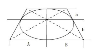
在挤压的过程中，对于远近平面的中间的某一个点，经过变化后会被推向远处
个人猜想：这个和画画时近大远小中间处被推向远处可能有关(即a<b)

完整的透视投影变换
$M_{persp}=M_{ortho}M_{persp\to ortho}$
如何定义截头体中较近的面 What’s near plane’s l, r, b, t
- 垂直可视角度 Vertical Field-of-View (fovY)
- 宽高比 Aspect ratio
- 垂直可视角度、宽高比和l, r, b, t的转换关系 How to convert from fovY and aspect to l, r, b, t?

$\tan \frac { f o v Y } { 2 } = \frac { t } { | n | },\quad aspect=\frac{r}{t}$

GAMES101笔记_Lec03~04_变换 Transform

1 为什么学习变换 Why study transformation

1.1 模型变换 Modeling

1.2 视图变换 Viewing

2 二维变换 2D Transformations

2.1 缩放变换矩阵 Scale Matrix

2.2 对称变换矩阵 Reflection Matrix

2.3 切变变换矩阵 Shear Matrix

2.4 旋转变换矩阵(默认绕原点、逆时针方向) Rotation Matrix

2.5 线性变换 Linear Transforms

3 齐次坐标 Homogeneous Coordinates

3.1 为什么学习齐次坐标 Why homogeneous coordinates

3.2 通过齐次坐标解决问题 Solution: Homogenous Coordinates

3.2.1 添加第三个坐标 Add a third coordinate (w-coordinate)

3.2.2 平移的矩阵表示 Matrix representation of translations

3.2.3 如果平移的是一个向量？ What if you translate a vector?

3.2.4 齐次坐标的妙处

3.2.5 仿射变换 Affine Transformations

3.2.6 使用齐次坐标的2D变换 2D Transformations

4 逆变换 Inverse Transform

5 组合变换 Composite Transform

5.1 变换的顺序会影响结果！ Transform Ordering Matters!

5.2 组合变换 Composite Transform

6 分解复杂的变换 Decomposing Complex Transforms

7 三维变换 3D Transformations

7.1 使用齐次坐标描述三维空间中的点和向量

7.2 三维空间中的缩放与平移 Scale and Translation

7.3 三维空间中的旋转 3D Rotations

7.3.1 沿x，y，z轴旋转 Rotation around x-, y-, or z-axis

7.3.2 任意一个旋转能看作几个绕轴旋转的组合 Compose any 3D rotation from Rx, Ry, Rz

8 观测变换 Viewing transformation

8.1 视图变换 View/Camera transformation

8.1.1 什么是视图变换 What is view transformation?

8.1.2 如何确定视图变换 How to perform view transformation?

8.1.3 标准位置 Key observation

8.2 投影变换 Projection transformation

8.2.1正交投影与透视投影 Perspective projection vs. orthographic projection

8.2.2 正交投影 Othographic projection

简单的理解 A simple way of understanding

正式的理解 In general

8.2.3 透视投影 Perspective projection

怎样做透视投影？

“挤压”变换的矩阵推导过程

猜你喜欢