搭建一个卷积神经网络

虽然对机器学习算法、神经网络、深度学习的接触也已经有一年了，但是还没有认真搭建过一个网络。为了帮助自己更好地理解，同时提高实践能力，自己动手搭建一个卷积神经网络，以备后面的学习使用。

使用比较熟悉的MNIST数据集，下载地址

包含四个部分

Training set images: train-images-idx3-ubyte.gz

Training set labels: train-labels-idx1-ubyte.gz

Test set images: t10k-images-idx3-ubyte.gz

Test set labels: t10k-labels-idx1-ubyte.gz

参考博客1：手把手教你用 TensorFlow 实现卷积神经网络（附代码）

参考博文2：深度学习四：tensorflow-使用卷积神经网络识别手写数字

为了方便自己理解，所以加了很多的注释。

# CNN.py
import tensorflow as tf
from tensorflow.examples.tutorials.mnist import input_data
sess = tf.InteractiveSession()

# 读取数据集
mnist = input_data.read_data_sets("MNIST_data/", one_hot=True)

# 函数申明
def weight_variable(shape):
    # 正态分布，标准差为0.1，默认最大为1，最小为-1，均值为0
    initial = tf.truncated_normal(shape, stddev=0.1)
    return tf.Variable(initial)
def bias_variable(shape):
    # 创建一个结构为shape矩阵也可以说是数组shape声明其行列，初始化所有值为0.1
    initial = tf.constant(0.1, shape == shape)
    return tf.Variable(initial)
def conv2d(x, W):
    # 卷积遍历各方向步数为1，SAME：边缘外自动补0，遍历相乘
    # padding 一般只有两个值
    return tf.nn.conv2d(x, W, strides=[1, 1, 1, 1], padding='SAME')
def max_pool_2x2(x):
    # 池化卷积结果（conv2d）池化层采用kernel大小为2*2，步数也为2，SAME：周围补0，取最大值。数据量缩小了4倍
    # x 是 CNN 第一步卷积的输出量，其shape必须为[batch, height, weight, channels];
    # ksize 是池化窗口的大小， shape为[batch, height, weight, channels]
    # stride 步长，一般是[1，stride， stride，1]
    return tf.nn.max_pool(x, ksize=[1, 2, 2, 1], strides=[1, 2, 2, 1], padding='SAME')


# 定义输入输出结构
# 可以理解为形参，用于定义过程，执行时再赋值
# dtype 是数据类型，常用的是tf.float32,tf.float64等数值类型
# shape是数据形状，默认None表示输入图片的数量不定，28*28图片分辨率
xs = tf.placeholder(tf.float32, [None, 28*28])
# 类别是0-9总共10个类别，对应输出分类结果
ys = tf.placeholder(tf.float32, [None, 10])

keep_prob = tf.placeholder(tf.float32)
# x_image又把xs reshape成了28*28*1的形状，灰色图片的通道是1.作为训练时的input，-1代表图片数量不定
x_image = tf.reshape(xs, [-1, 28, 28, 1])


# 搭建网络
# 第一层卷积池化
# 第一二参数值得卷积核尺寸大小，即patch
w_conv1 = weight_variable([5, 5, 1, 32])
b_conv1 = bias_variable([32])   # 32个偏置值
h_conv1 = tf.nn.relu(conv2d(x_image, w_conv1)+b_conv1)  # 得到28*28*32
h_pool1 = max_pool_2x2(h_conv1)  # 得到14*14*32

# 第二层卷积池化
# 第三个参数是图像通道数，第四个参数是卷积核的数目，代表会出现多少个卷积特征图像;
w_conv2 = weight_variable([5, 5, 32, 64])
b_conv2 = bias_variable([64])
h_conv2 = tf.nn.relu(conv2d(h_pool1, w_conv2)+b_conv2)  # 得到14*14*64
h_pool2 = max_pool_2x2(h_conv2)  # 得到7*7*64

# 第三层全连接层
w_fc1 = weight_variable([7*7*64, 1024])
b_fc1 = bias_variable([1024])
# 将第二层卷积池化结果reshape成只有一行7*7*64个数据
# [n_samples, 7, 7, 64] == [n_samples, 7 * 7 * 64]
h_pool2_flat = tf.reshape(h_pool2, [-1, 7*7*64])
# 卷积操作，结果是1*1*1024，单行乘以单列等于1*1矩阵，matmul实现最基本的矩阵相乘
# 不同于tf.nn.conv2d的遍历相乘，自动认为是前行向量后列向量
h_fc1 = tf.nn.relu(tf.matmul(h_pool2_flat, w_fc1)+ b_fc1)

# 对卷积结果执行dropout操作
h_fc1_dropout = tf.nn.dropout(h_fc1, keep_prob)

# 第四层输出操作
# 二维张量，1*1024矩阵卷积，共10个卷积，对应ys长度为10
w_fc2 = weight_variable([1024, 10])
b_fc2 = bias_variable([10])
y_conv = tf.nn.softmax(tf.matmul(h_fc1_dropout, w_fc2)+b_fc2)

# 定义损失函数
cross_entropy = tf.reduce_mean(-tf.reduce_sum(ys*tf.log(y_conv), reduction_indices=[1]))
# AdamOptimizer通过使用动量（参数的移动平均数）来改善传统梯度下降，促进超参数动态调整
train_step = tf.train.AdamOptimizer(1e-4).minimize(cross_entropy)

# 训练验证
tf.global_variables_initializer().run()
# tf.equal(A, B)是对比这两个矩阵或者向量的相等的元素，如果相等返回True，否则返回False，返回的值的矩阵维度和A是一样的
correct_prediction = tf.equal(tf.argmax(y_conv, 1), tf.argmax(ys, 1))
# print(correct_prediction)
# tf.arg_max(input, axis=None, name=None, dimension=None) 是对矩阵按行或列计算最大值（axis：0表示按列，1表示按行）
accuracy = tf.reduce_mean(tf.cast(correct_prediction, tf.float32))  # 数据类型转换

for i in range(1500):
    batch_x, batch_y = mnist.train.next_batch(50)
    if i%100 == 0:
        train_accuracy = accuracy.eval(feed_dict={xs:batch_x, ys:batch_y, keep_prob: 1.0})
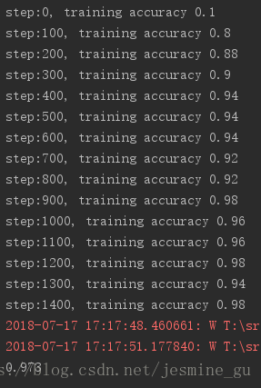
        print('step:%d, training accuracy %g' %(i, train_accuracy))
    train_step.run(feed_dict={xs:batch_x, ys:batch_y, keep_prob:0.5})

print(accuracy.eval({xs:mnist.test.images, ys:mnist.test.labels, keep_prob:1.0}))

运行结果

除了Adam算法的优化器外，tensorflow还提供了一些优化器，比如： 

class tf.train.GradientDescentOptimizer–梯度下降算法的优化器 

class tf.train.AdadeltaOptimizer – 使用adadelta算法的优化器 

class tf.train.AdagradOptimizer – 使用adagradOptimizer算法的优化器 

class tf.train.MomentumOptimizer – 使用Momentum算法的优化器 

把激活函数换成sigmoid试了一下

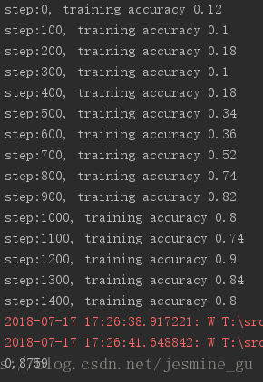
可以看到sigmoid的效果没有ReLU好

添加一个卷积池化层

# CNN.py
import tensorflow as tf
from tensorflow.examples.tutorials.mnist import input_data
sess = tf.InteractiveSession()


# 函数申明
def weight_variable(shape):
    # 正态分布，标准差为0.1，默认最大为1，最小为-1，均值为0
    initial = tf.truncated_normal(shape, stddev=0.1)
    return tf.Variable(initial)
def bias_variable(shape):
    # 创建一个结构为shape矩阵也可以说是数组shape声明其行列，初始化所有值为0.1
    initial = tf.constant(0.1, shape == shape)
    return tf.Variable(initial)
def conv2d(x, W):
    # 卷积遍历各方向步数为1，SAME：边缘外自动补0，遍历相乘
    # padding 一般只有两个值
    return tf.nn.conv2d(x, W, strides=[1, 1, 1, 1], padding='SAME')
def max_pool_2x2(x):
    # 池化卷积结果（conv2d）池化层采用kernel大小为2*2，步数也为2，SAME：周围补0，取最大值。数据量缩小了4倍
    # x 是 CNN 第一步卷积的输出量，其shape必须为[batch, height, weight, channels];
    # ksize 是池化窗口的大小， shape为[batch, height, weight, channels]
    # stride 步长，一般是[1，stride， stride，1]
    return tf.nn.max_pool(x, ksize=[1, 2, 2, 1], strides=[1, 2, 2, 1], padding='SAME')

def deep_CNN(xs):
    # x_image又把xs reshape成了28*28*1的形状，灰色图片的通道是1.作为训练时的input，-1代表图片数量不定
    x_image = tf.reshape(xs, [-1, 28, 28, 1])

    # 搭建网络
    # 第一层卷积池化
    # 第一二参数值得卷积核尺寸大小，即patch
    w_conv1 = weight_variable([5, 5, 1, 32])
    b_conv1 = bias_variable([32])   # 32个偏置值
    h_conv1 = tf.nn.relu(conv2d(x_image, w_conv1)+b_conv1)  # 得到28*28*32
    #h_conv1 = tf.nn.sigmoid(conv2d(x_image, w_conv1)+b_conv1)
    h_pool1 = max_pool_2x2(h_conv1)  # 得到14*14*32

    # 第二层卷积池化
    # 第三个参数是图像通道数，第四个参数是卷积核的数目，代表会出现多少个卷积特征图像;
    w_conv2 = weight_variable([5, 5, 32, 64])
    b_conv2 = bias_variable([64])
    h_conv2 = tf.nn.relu(conv2d(h_pool1, w_conv2)+b_conv2)  # 得到14*14*64
    #h_conv2 = tf.nn.sigmoid(conv2d(h_pool1, w_conv2)+b_conv2)
    h_pool2 = max_pool_2x2(h_conv2)  # 得到7*7*64

    # 添加一层卷积池化层
    w_conv3 = weight_variable([5, 5, 64, 128])
    b_conv3 = bias_variable([128])
    h_conv3 = tf.nn.relu(conv2d(h_pool2, w_conv3)+b_conv3)  # 得到7*7*128
    #h_conv3 = tf.nn.sigmoid(conv2d(h_pool1, w_conv2)+b_conv2)
    h_pool3 = max_pool_2x2(h_conv3)  # 得到4*4*128

    # 第四层全连接层
    w_fc1 = weight_variable([4*4*128, 1024])
    b_fc1 = bias_variable([1024])
    # 将第三层卷积池化结果reshape成只有一行7*7*128个数据
    # [n_samples, 4, 4, 128] == [n_samples, 4 * 4 * 128]
    h_pool3_flat = tf.reshape(h_pool3, [-1, 4*4*128])
    # -1 表示不知道该填什么数字合适的情况下，可以选择
    # 卷积操作，结果是1*1*1024，单行乘以单列等于1*1矩阵，matmul实现最基本的矩阵相乘
    # 不同于tf.nn.conv2d的遍历相乘，自动认为是前行向量后列向量
    h_fc1 = tf.nn.relu(tf.matmul(h_pool3_flat, w_fc1)+ b_fc1)
    #h_fc1 = tf.nn.sigmoid(tf.matmul(h_pool2_flat, w_fc1)+ b_fc1)

    # 对卷积结果执行dropout操作
    keep_prob = tf.placeholder(tf.float32)
    h_fc1_dropout = tf.nn.dropout(h_fc1, keep_prob)
    # tf.nn.dropout(x, keep_prob, noise_shape=None, seed=None, name=None)
    # 第二个参数keep_prob: 设置神经元被选中的概率,在初始化时keep_prob是一个占位符

    # 第四层输出操作
    # 二维张量，1*1024矩阵卷积，共10个卷积，对应ys长度为10
    w_fc2 = weight_variable([1024, 10])
    b_fc2 = bias_variable([10])
    y_conv = tf.nn.softmax(tf.matmul(h_fc1_dropout, w_fc2)+b_fc2)

    return y_conv, keep_prob

def main():
    # 读取数据集
    mnist = input_data.read_data_sets("MNIST_data/", one_hot=True)

    # 定义输入输出结构
    # tf.placeholder可以理解为形参，用于定义过程，执行时再赋值
    # dtype 是数据类型，常用的是tf.float32,tf.float64等数值类型
    # shape是数据形状，默认None表示输入图片的数量不定，28*28图片分辨率
    xs = tf.placeholder(tf.float32, [None, 28 * 28])
    # 类别是0-9总共10个类别，对应输出分类结果
    ys = tf.placeholder(tf.float32, [None, 10])

    y_conv, keep_prob = deep_CNN(xs)

    # 定义损失函数
    # cross_entropy = tf.reduce_mean(-tf.reduce_sum(ys*tf.log(y_conv), reduction_indices=[1]))
    cross_entropy = tf.reduce_mean(tf.nn.softmax_cross_entropy_with_logits(labels=ys, logits=y_conv))
    # AdamOptimizer通过使用动量（参数的移动平均数）来改善传统梯度下降，促进超参数动态调整
    train_step = tf.train.AdamOptimizer(1e-4).minimize(cross_entropy)

    # 训练验证
    # tf.equal(A, B)是对比这两个矩阵或者向量的相等的元素，如果相等返回True，否则返回False，返回的值的矩阵维度和A是一样的
    correct_prediction = tf.equal(tf.argmax(y_conv, 1), tf.argmax(ys, 1))
    # print(correct_prediction)
    # tf.arg_max(input, axis=None, name=None, dimension=None) 是对矩阵按行或列计算最大值（axis：0表示按列，1表示按行）
    accuracy = tf.reduce_mean(tf.cast(correct_prediction, tf.float32))  # 数据类型转换

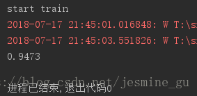
    print("start train")
    sess.run(tf.global_variables_initializer())

    for i in range(1500):
        batch_x, batch_y = mnist.train.next_batch(50)
        if i % 100 == 0:
            train_accuracy = accuracy.eval(feed_dict={xs: batch_x, ys: batch_y, keep_prob: 1.0})
            print('step:%d, training accuracy %g' % (i, train_accuracy))
        train_step.run(feed_dict={xs: batch_x, ys: batch_y, keep_prob: 0.5})

    # 测试
    print(accuracy.eval({xs: mnist.test.images, ys: mnist.test.labels, keep_prob: 1.0}))

if __name__ == '__main__':
    main()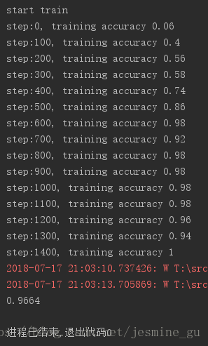

结果看来没太大差别，效果没有什么提升

接下来保存和恢复参数

为了方便调试，节省训练时间，我把迭代次数调到了1000

训练时

    saver = tf.train.Saver()

    sess.run(tf.global_variables_initializer())

    for i in range(1000):
        batch_x, batch_y = mnist.train.next_batch(50)
        if i % 100 == 0:
            train_accuracy = accuracy.eval(feed_dict={xs: batch_x, ys: batch_y, keep_prob: 1.0})
            print('step:%d, training accuracy %g' % (i, train_accuracy))
        train_step.run(feed_dict={xs: batch_x, ys: batch_y, keep_prob: 0.5})
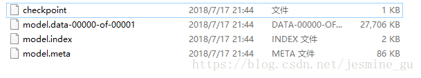
        saver.save(sess, "input_data/model")
   

得到的文件

测试时

    saver = tf.train.Saver()

    sess.run(tf.global_variables_initializer())
    
    saver.restore(sess, "input_data/model")
    # 测试
    print(accuracy.eval({xs: mnist.test.images, ys: mnist.test.labels, keep_prob: 1.0}))

直接得到测试结果

还需继续改进

未完待续......