文章目录

一、卷积神经网络
二、环境配置及数据集准备
三、猫狗数据分类建模

一、卷积神经网络

卷积神经网络（Convolutional Neural Networks, CNN 是一类包含卷积计算且具有深度结构的前馈神经网络（Feedforward Neural Networks），是深度学习（deep learning）的代表算法之一。卷积神经网络具有表征学习（representation learning）能力，能够按其阶层结构对输入信息进行平移不变分类（shift-invariant classification），因此也被称为“平移不变人工神经网络（Shift-Invariant Artificial Neural Networks, SIANN）”

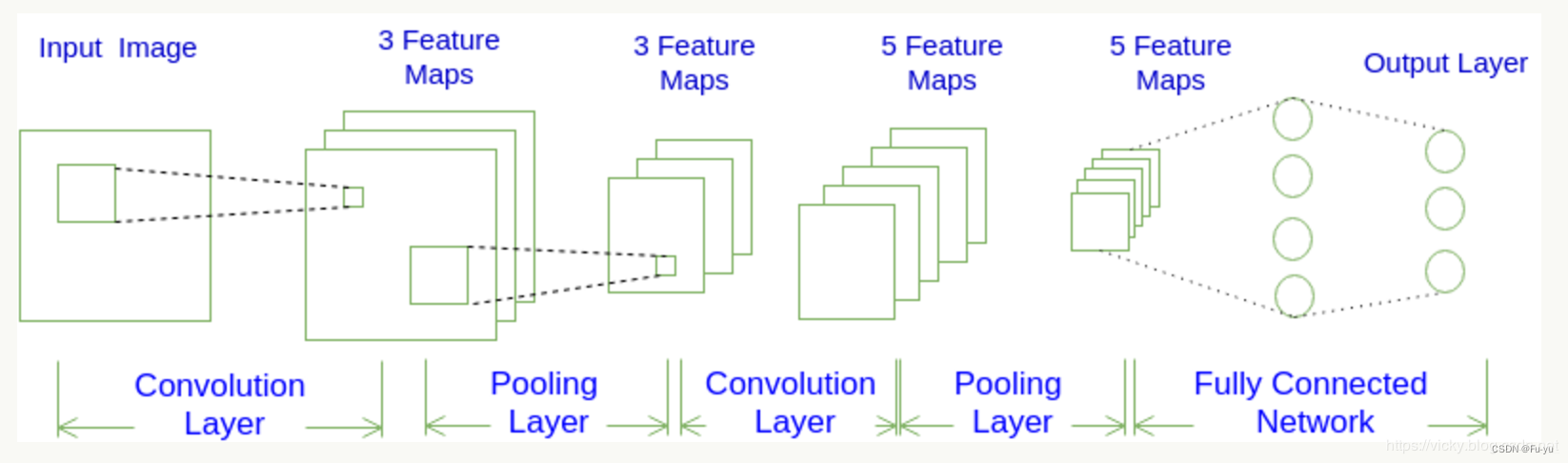
卷积神经网络CNN的结构一般包含这几个层：

输入层：用于数据的输入
卷积层：使用卷积核进行特征提取和特征映射
激励层：由于卷积也是一种线性运算，因此需要增加非线性映射
池化层：进行下采样，对特征图稀疏处理，减少数据运算量
全连接层：通常在CNN的尾部进行重新拟合，减少特征信息的损失

在这里插入图片描述
CNN的三个特点：

局部连接：这个是最容易想到的，每个神经元不再和上一层的所有神经元相连，而只和一小部分神经元相连。这样就减少了很多参数
权值共享：一组连接可以共享同一个权重，而不是每个连接有一个不同的权重，这样又减少了很多参数。
下采样：可以使用Pooling来减少每层的样本数，进一步减少参数数量，同时还可以提升模型的鲁棒性。

卷积层：
如图是33的卷积核（卷积核一般采用33和2*2 ）与上一层的结果（输入层）进行卷积的过程
在这里插入图片描述
池化层：

在卷积层进行特征提取后，输出的特征图会被传递至池化层进行特征选择和信息过滤。
池化层包含预设定的池化函数，其功能是将特征图中单个点的结果替换为其相邻区域的特征图统计量。
池化层选取池化区域与卷积核扫描特征图步骤相同，由池化大小、步长和填充控制。

在这里插入图片描述
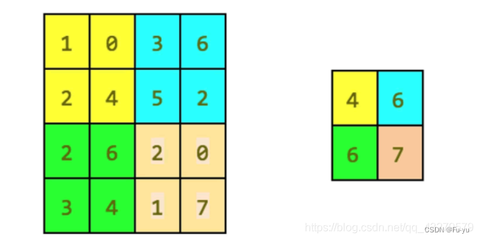
最大池化，它只是输出在区域中观察到的最大输入值
均值池化，它只是输出在区域中观察到的平均输入值
两者最大区别在于卷积核的不同（池化是一种特殊的卷积过程）。

全连接层：
在这里插入图片描述

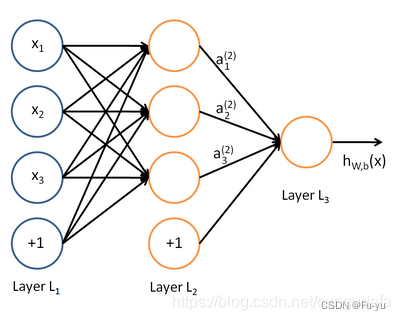
全连接层位于卷积神经网络隐含层的最后部分，并只向其它全连接层传递信号。
特征图在全连接层中会失去空间拓扑结构，被展开为向量并通过激励函数。
全连接层的作用则是对提取的特征进行非线性组合以得到输出，即全连接层本身不被期望具有特征提取能力，而是试图利用现有的高阶特征完成学习目标。

输出层：

卷积神经网络中输出层的上游通常是全连接层，因此其结构和工作原理与传统前馈神经网络中的输出层相同。
对于图像分类问题，输出层使用逻辑函数或归一化指数函数（softmax function）输出分类标签。
在物体识别（object detection）问题中，输出层可设计为输出物体的中心坐标、大小和分类。
在图像语义分割中，输出层直接输出每个像素的分类结果。

二、环境配置及数据集准备

配置TensorFlow、Keras
打开 cmd 命令终端，创建虚拟环境。

conda create -n tf1 python=3.6
#tf1是自己为创建虚拟环境取的名字，后面python的版本可以根据自己需求进行选择

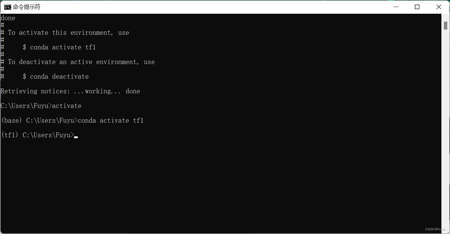
激活环境：

activate
conda activate tf1

在这里插入图片描述
安装tensorflow和keras：

pip install -i https://pypi.tuna.tsinghua.edu.cn/simple tensorflow==1.14.0
pip install -i https://pypi.tuna.tsinghua.edu.cn/simple keras==2.2.5

安装 nb_conda_kernels 包

conda install nb_conda_kernels

数据集的下载
kaggle网站的数据集下载地址：
https://www.kaggle.com/lizhensheng/-2000

三、猫狗数据分类建模

1、猫狗图像预处理

代码如下：

import tensorflow as tf
import keras
import os, shutil 
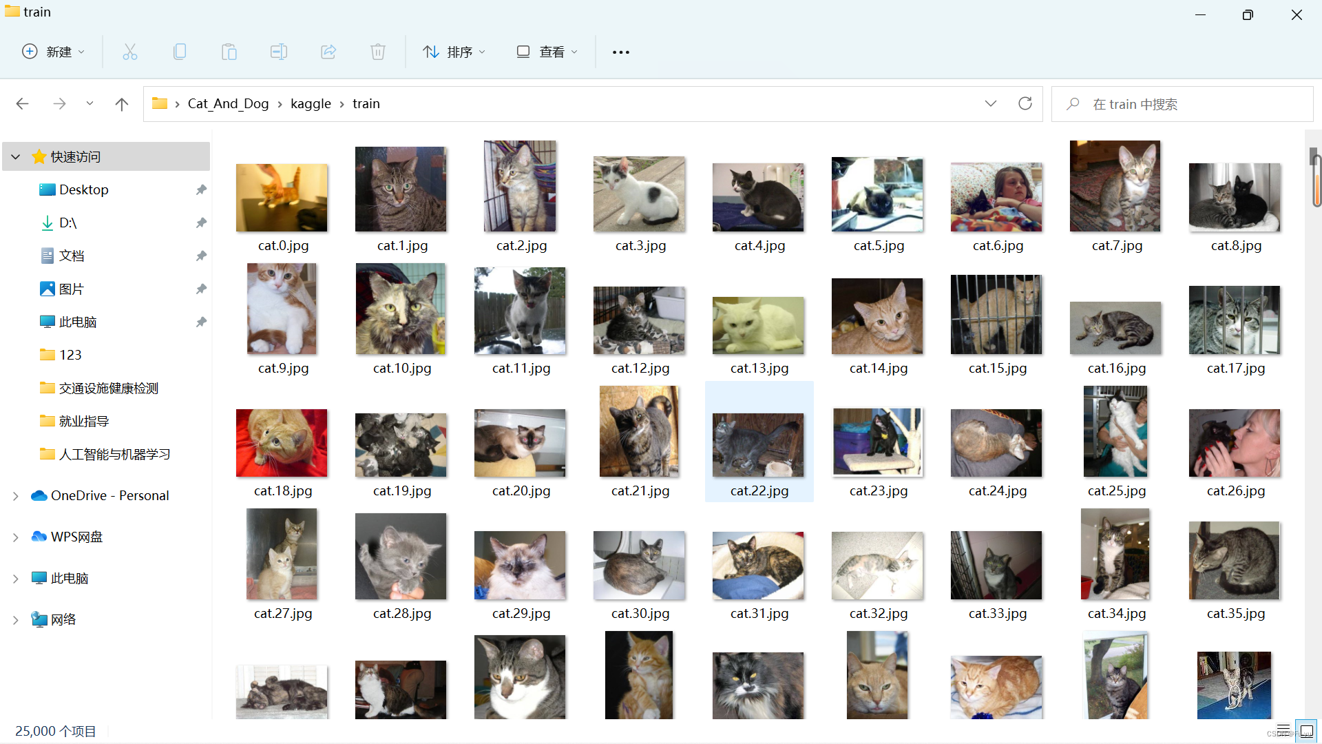
# 原始目录所在的路径
original_dataset_dir = 'D:\\Desktop\\Cat_And_Dog\\kaggle\\train\\'

# 数据集分类后的目录
base_dir = 'D:\\Desktop\\Cat_And_Dog\\kaggle\\cats_and_dogs_small'
os.mkdir(base_dir)

# # 训练、验证、测试数据集的目录
train_dir = os.path.join(base_dir, 'train')
os.mkdir(train_dir)
validation_dir = os.path.join(base_dir, 'validation')
os.mkdir(validation_dir)
test_dir = os.path.join(base_dir, 'test')
os.mkdir(test_dir)

# 猫训练图片所在目录
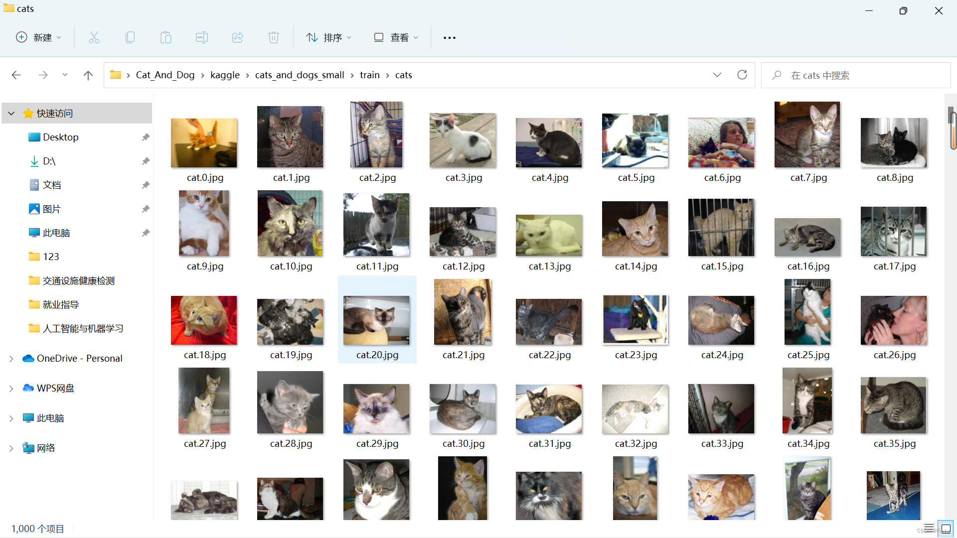
train_cats_dir = os.path.join(train_dir, 'cats')
os.mkdir(train_cats_dir)

# 狗训练图片所在目录
train_dogs_dir = os.path.join(train_dir, 'dogs')
os.mkdir(train_dogs_dir)

# 猫验证图片所在目录
validation_cats_dir = os.path.join(validation_dir, 'cats')
os.mkdir(validation_cats_dir)

# 狗验证数据集所在目录
validation_dogs_dir = os.path.join(validation_dir, 'dogs')
os.mkdir(validation_dogs_dir)

# 猫测试数据集所在目录
test_cats_dir = os.path.join(test_dir, 'cats')
os.mkdir(test_cats_dir)

# 狗测试数据集所在目录
test_dogs_dir = os.path.join(test_dir, 'dogs')
os.mkdir(test_dogs_dir)

# 将前1000张猫图像复制到train_cats_dir
fnames = ['cat.{}.jpg'.format(i) for i in range(1000)]
for fname in fnames:
    src = os.path.join(original_dataset_dir, fname)
    dst = os.path.join(train_cats_dir, fname)
    shutil.copyfile(src, dst)

# 将下500张猫图像复制到validation_cats_dir
fnames = ['cat.{}.jpg'.format(i) for i in range(1000, 1500)]
for fname in fnames:
    src = os.path.join(original_dataset_dir, fname)
    dst = os.path.join(validation_cats_dir, fname)
    shutil.copyfile(src, dst)
    
# 将下500张猫图像复制到test_cats_dir
fnames = ['cat.{}.jpg'.format(i) for i in range(1500, 2000)]
for fname in fnames:
    src = os.path.join(original_dataset_dir, fname)
    dst = os.path.join(test_cats_dir, fname)
    shutil.copyfile(src, dst)
    
# 将前1000张狗图像复制到train_dogs_dir
fnames = ['dog.{}.jpg'.format(i) for i in range(1000)]
for fname in fnames:
    src = os.path.join(original_dataset_dir, fname)
    dst = os.path.join(train_dogs_dir, fname)
    shutil.copyfile(src, dst)
    
# 将下500张狗图像复制到validation_dogs_dir
fnames = ['dog.{}.jpg'.format(i) for i in range(1000, 1500)]
for fname in fnames:
    src = os.path.join(original_dataset_dir, fname)
    dst = os.path.join(validation_dogs_dir, fname)
    shutil.copyfile(src, dst)
    
# 将下500张狗图像复制到test_dogs_dir
fnames = ['dog.{}.jpg'.format(i) for i in range(1500, 2000)]
for fname in fnames:
    src = os.path.join(original_dataset_dir, fname)
    dst = os.path.join(test_dogs_dir, fname)
    shutil.copyfile(src, dst)

分类前：
在这里插入图片描述
分类后：

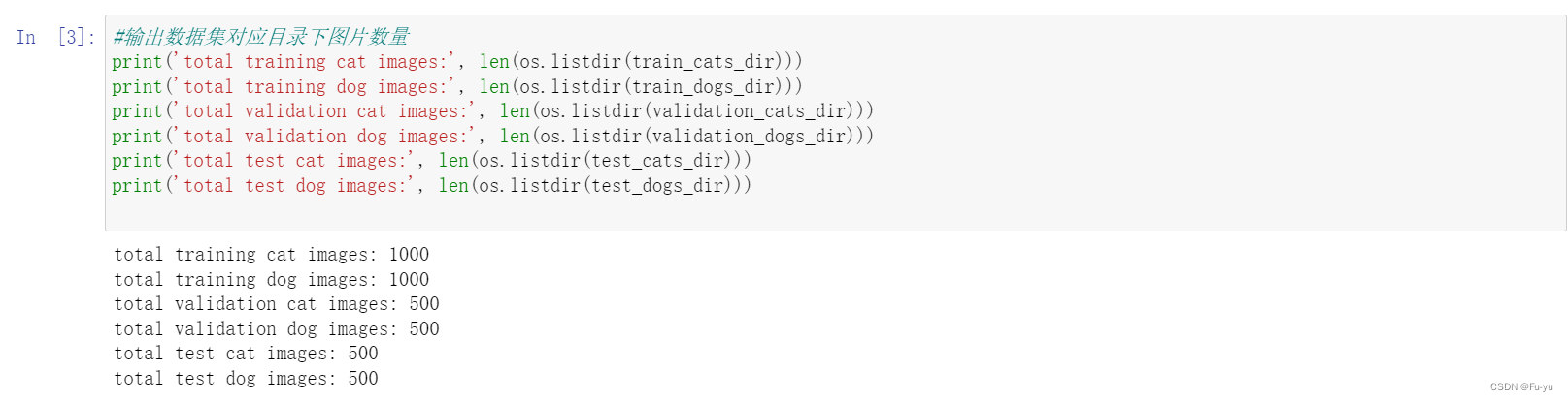
查看分类后，对应目录下图片数量

#输出数据集对应目录下图片数量
print('total training cat images:', len(os.listdir(train_cats_dir)))
print('total training dog images:', len(os.listdir(train_dogs_dir)))
print('total validation cat images:', len(os.listdir(validation_cats_dir)))
print('total validation dog images:', len(os.listdir(validation_dogs_dir)))
print('total test cat images:', len(os.listdir(test_cats_dir)))
print('total test dog images:', len(os.listdir(test_dogs_dir)))

在这里插入图片描述

2、猫狗分类的实例——基准模型

1、构建网络模型

#网络模型构建
from keras import layers
from keras import models
#keras的序贯模型
model = models.Sequential()
#卷积层，卷积核是3*3，激活函数relu
model.add(layers.Conv2D(32, (3, 3), activation='relu',
                        input_shape=(150, 150, 3)))
#最大池化层
model.add(layers.MaxPooling2D((2, 2)))
#卷积层，卷积核2*2，激活函数relu
model.add(layers.Conv2D(64, (3, 3), activation='relu'))
#最大池化层
model.add(layers.MaxPooling2D((2, 2)))
#卷积层，卷积核是3*3，激活函数relu
model.add(layers.Conv2D(128, (3, 3), activation='relu'))
#最大池化层
model.add(layers.MaxPooling2D((2, 2)))
#卷积层，卷积核是3*3，激活函数relu
model.add(layers.Conv2D(128, (3, 3), activation='relu'))
#最大池化层
model.add(layers.MaxPooling2D((2, 2)))
#flatten层，用于将多维的输入一维化，用于卷积层和全连接层的过渡
model.add(layers.Flatten())
#全连接，激活函数relu
model.add(layers.Dense(512, activation='relu'))
#全连接，激活函数sigmoid
model.add(layers.Dense(1, activation='sigmoid'))

查看模型各层的参数状况

#输出模型各层的参数状况
model.summary()

在这里插入图片描述
2、配置训练方法

model.compile(optimizer = 优化器，
              loss = 损失函数，
              metrics = ["准确率”])

其中，优化器和损失函数可以是字符串形式的名字，也可以是函数形式。

from keras import optimizers

model.compile(loss='binary_crossentropy',
              optimizer=optimizers.RMSprop(lr=1e-4),
              metrics=['acc'])

3、文件中图像转换成所需格式
将训练和验证的图片，调整为150*150

from keras.preprocessing.image import ImageDataGenerator

# 所有图像将按1/255重新缩放
train_datagen = ImageDataGenerator(rescale=1./255)
test_datagen = ImageDataGenerator(rescale=1./255)

train_generator = train_datagen.flow_from_directory(
        # 这是目标目录
        train_dir,
        # 所有图像将调整为150x150
        target_size=(150, 150),
        batch_size=20,
        # 因为我们使用二元交叉熵损失，我们需要二元标签
        class_mode='binary')

validation_generator = test_datagen.flow_from_directory(
        validation_dir,
        target_size=(150, 150),
        batch_size=20,
        class_mode='binary')

在这里插入图片描述
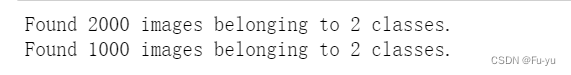
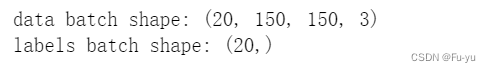
查看处理结果

#查看上面对于图片预处理的处理结果
for data_batch, labels_batch in train_generator:
    print('data batch shape:', data_batch.shape)
    print('labels batch shape:', labels_batch.shape)
    break

在这里插入图片描述
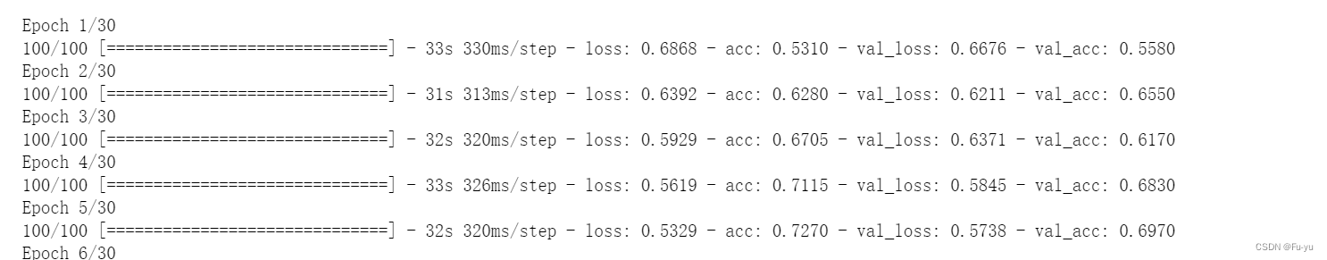
4、模型训练并保存生成的模型

#模型训练过程
history = model.fit_generator(
      train_generator,
      steps_per_epoch=100,
      epochs=30,
      validation_data=validation_generator,
      validation_steps=50)
#保存训练得到的的模型
model.save('D:\\Desktop\\Cat_And_Dog\\kaggle\\cats_and_dogs_small_1.h5')

在这里插入图片描述
5、结果可视化

#对于模型进行评估，查看预测的准确性
import matplotlib.pyplot as plt

acc = history.history['acc']
val_acc = history.history['val_acc']
loss = history.history['loss']
val_loss = history.history['val_loss']

epochs = range(len(acc))

plt.plot(epochs, acc, 'bo', label='Training acc')
plt.plot(epochs, val_acc, 'b', label='Validation acc')
plt.title('Training and validation accuracy')
plt.legend()

plt.figure()

plt.plot(epochs, loss, 'bo', label='Training loss')
plt.plot(epochs, val_loss, 'b', label='Validation loss')
plt.title('Training and validation loss')
plt.legend()

plt.show()

在这里插入图片描述

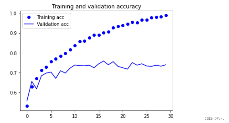
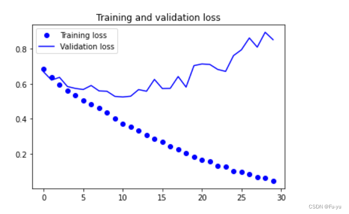
由可视化结果，可以发现训练的loss是成上升趋势，模型过拟合。

过拟合：
过拟合（overfitting）是指模型在训练集上表现很好，但在测试集或未见过的数据上表现较差的情况。
过拟合的原因可能包括：

模型复杂度过高：过于复杂的模型可以灵活地适应训练数据中的噪声和异常，但泛化能力较差。
数据噪声：训练集中存在大量噪声或异常值，导致模型过度拟合这些不代表真实规律的数据。
数据量过少：当训练集的样本数量较少时，模型容易记忆住训练数据的细节而无法泛化到新样本。

避免过拟合的方法包括：

简化模型：降低模型的复杂度，减少模型的参数量，限制模型的学习能力。
数据清洗：去除异常值和噪声，确保训练数据的质量。
数据增强：通过旋转、缩放、平移等方式扩充训练数据，增加样本的多样性。
正则化技术：如L1、L2正则化，通过对模型参数的约束，减小模型的过拟合风险。
交叉验证：使用交叉验证来评估模型在不同数据集上的性能，选择表现最好的模型。

数据增强：

数据增强是在机器学习和深度学习中一种常用的技术，用于扩充训练数据集的大小和多样性。通过对原始数据进行一系列的随机变换和合成操作，可以生成与原始数据具有相似特征但又稍有差异的新样本。数据增强的目的在于提高模型的鲁棒性和泛化能力，减少过拟合现象。通过引入更多的变化和多样性，模型可以更好地学习到数据的各种特征和变化模式，从而提高其在真实世界中的适应能力。

常见的数据增强技术包括但不限于以下几种：

随机翻转：例如图像的水平或垂直翻转，可以扩充数据集，并对模型具有平移不变性的任务（如物体识别）有帮助。
随机裁剪和缩放：通过随机裁剪和缩放图像，可以模拟不同的尺度和视角，增加数据的多样性，并改善模型对于目标的检测和识别能力。
随机旋转和仿射变换：对于图像数据，进行随机旋转、平移、缩放和倾斜等仿射变换，可以增加数据的多样性，提高模型对于旋转、平移和形变等变化的鲁棒性。
增加噪声：向数据中添加随机噪声，如高斯噪声、椒盐噪声等，可以提高模型对于噪声环境下的稳定性和鲁棒性。
数据mixup：将两个或多个不同的样本进行线性组合，生成新的样本。这样可以使得模型对于不同类别之间的边界更加清晰，从而提高泛化性能。

3、基准模型的调整

1、图像增强
利用图像生成器定义一些常见的图像变换，图像增强就是通过对于图像进行变换，从而，增强图像中的有用信息。

#该部分代码及以后的代码，用于替代基准模型中分类后面的代码（执行代码前，需要先将之前分类的目录删掉，重写生成分类，否则，会发生错误）
from keras.preprocessing.image import ImageDataGenerator
datagen = ImageDataGenerator(
      rotation_range=40,
      width_shift_range=0.2,
      height_shift_range=0.2,
      shear_range=0.2,
      zoom_range=0.2,
      horizontal_flip=True,
      fill_mode='nearest')

①rotation_range
一个角度值(0-180)，在这个范围内可以随机旋转图片
②width_shift和height_shift
范围(作为总宽度或高度的一部分)，在其中可以随机地垂直或水平地转换图片
③shear_range
用于随机应用剪切转换
④zoom_range
用于在图片内部随机缩放
⑤horizontal_flip
用于水平随机翻转一半的图像——当没有假设水平不对称时(例如真实世界的图片)
⑥fill_mode
用于填充新创建像素的策略，它可以在旋转或宽度/高度移动之后出现

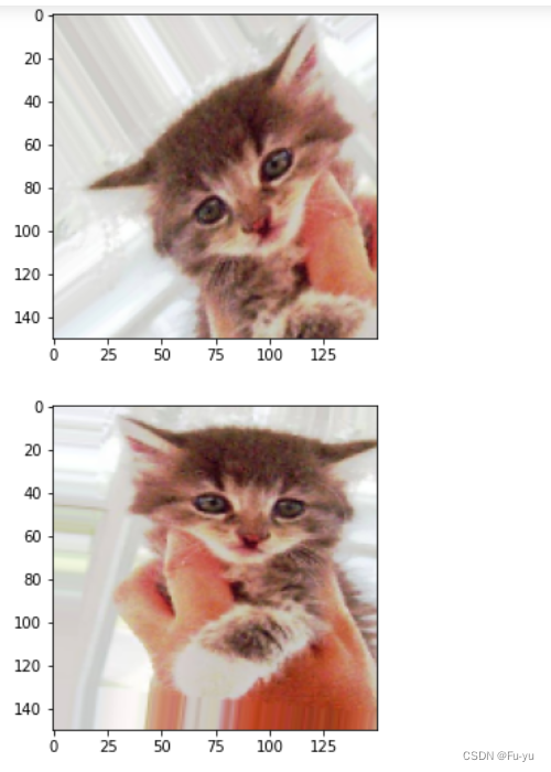
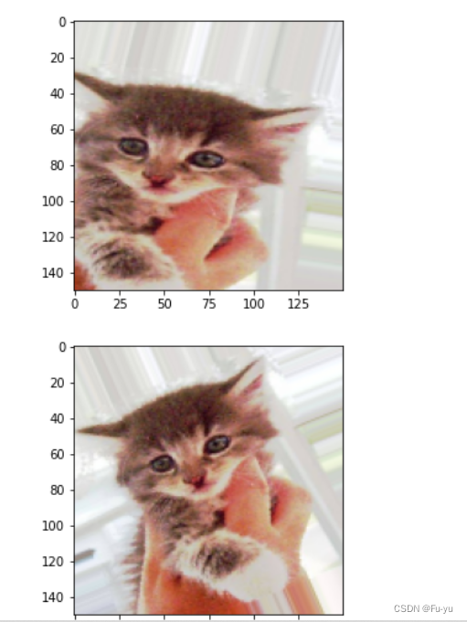
2、查看增强后的图像

import matplotlib.pyplot as plt
# This is module with image preprocessing utilities
from keras.preprocessing import image
fnames = [os.path.join(train_cats_dir, fname) for fname in os.listdir(train_cats_dir)]
# We pick one image to "augment"
img_path = fnames[3]
# Read the image and resize it
img = image.load_img(img_path, target_size=(150, 150))
# Convert it to a Numpy array with shape (150, 150, 3)
x = image.img_to_array(img)
# Reshape it to (1, 150, 150, 3)
x = x.reshape((1,) + x.shape)
# The .flow() command below generates batches of randomly transformed images.
# It will loop indefinitely, so we need to `break` the loop at some point!
i = 0
for batch in datagen.flow(x, batch_size=1):
    plt.figure(i)
    imgplot = plt.imshow(image.array_to_img(batch[0]))
    i += 1
    if i % 4 == 0:
        break
plt.show()

在这里插入图片描述

3、网络模型增加一层dropout

#网络模型构建
from keras import layers
from keras import models
#keras的序贯模型
model = models.Sequential()
#卷积层，卷积核是3*3，激活函数relu
model.add(layers.Conv2D(32, (3, 3), activation='relu',
                        input_shape=(150, 150, 3)))
#最大池化层
model.add(layers.MaxPooling2D((2, 2)))
#卷积层，卷积核2*2，激活函数relu
model.add(layers.Conv2D(64, (3, 3), activation='relu'))
#最大池化层
model.add(layers.MaxPooling2D((2, 2)))
#卷积层，卷积核是3*3，激活函数relu
model.add(layers.Conv2D(128, (3, 3), activation='relu'))
#最大池化层
model.add(layers.MaxPooling2D((2, 2)))
#卷积层，卷积核是3*3，激活函数relu
model.add(layers.Conv2D(128, (3, 3), activation='relu'))
#最大池化层
model.add(layers.MaxPooling2D((2, 2)))
#flatten层，用于将多维的输入一维化，用于卷积层和全连接层的过渡
model.add(layers.Flatten())
#退出层
model.add(layers.Dropout(0.5))
#全连接，激活函数relu
model.add(layers.Dense(512, activation='relu'))
#全连接，激活函数sigmoid
model.add(layers.Dense(1, activation='sigmoid'))
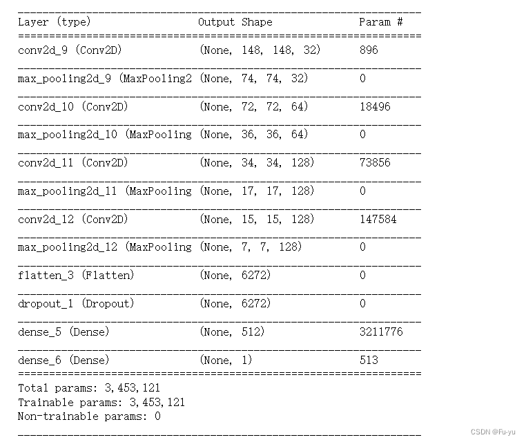
#输出模型各层的参数状况
model.summary()
from keras import optimizers

model.compile(loss='binary_crossentropy',
              optimizer=optimizers.RMSprop(lr=1e-4),
              metrics=['acc'])

添加dropout后的网络结构
在这里插入图片描述

4、训练模型

train_datagen = ImageDataGenerator(
    rescale=1./255,
    rotation_range=40,
    width_shift_range=0.2,
    height_shift_range=0.2,
    shear_range=0.2,
    zoom_range=0.2,
    horizontal_flip=True,)
# Note that the validation data should not be augmented!
test_datagen = ImageDataGenerator(rescale=1./255)
train_generator = train_datagen.flow_from_directory(
        # This is the target directory
        train_dir,
        # All images will be resized to 150x150
        target_size=(150, 150),
        batch_size=32,
        # Since we use binary_crossentropy loss, we need binary labels
        class_mode='binary')
validation_generator = test_datagen.flow_from_directory(
        validation_dir,
        target_size=(150, 150),
        batch_size=32,
        class_mode='binary')
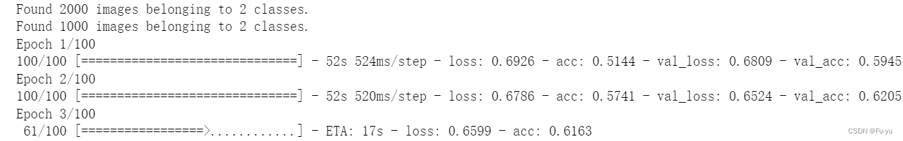
history = model.fit_generator(
      train_generator,
      steps_per_epoch=100,
      epochs=100,
      validation_data=validation_generator,
      validation_steps=50)
model.save('D:\\Desktop\\Cat_And_Dog\\kaggle\\cats_and_dogs_small_2.h5')

在这里插入图片描述
5、结果可视化

acc = history.history['acc']
val_acc = history.history['val_acc']
loss = history.history['loss']
val_loss = history.history['val_loss']
epochs = range(len(acc))
plt.plot(epochs, acc, 'bo', label='Training acc')
plt.plot(epochs, val_acc, 'b', label='Validation acc')
plt.title('Training and validation accuracy')
plt.legend()
plt.figure()
plt.plot(epochs, loss, 'bo', label='Training loss')
plt.plot(epochs, val_loss, 'b', label='Validation loss')
plt.title('Training and validation loss')
plt.legend()
plt.show()

在这里插入图片描述
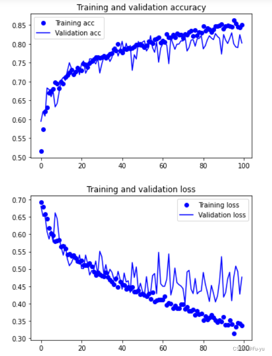
可以发现训练曲线更加紧密地跟踪验证曲线，波动的幅度也降低了些，训练效果更好了。

总结
通过使用TensorFlow和Keras搭建卷积神经网络完成狗猫数据集的分类实验，我深刻理解到了数据预处理、模型设计和超参数选择对于模型性能的重要影响。这个实验为我进一步深入学习和应用深度学习提供了宝贵的经验和启示。

参考链接
【TensorFlow&Keras】入门猫狗数据集实验–理解卷积神经网络CNN
基于Tensorflow和Keras实现卷积神经网络CNN

基于卷积神经网络的目标分类案例