深度学习——基于卷积神经网络的宝石分类

 ​活动地址：CSDN21天学习挑战赛

数据集下载

可以在百度飞桨AI Studio中下载数据集，下载地址如下：

宝石数据集（Gemstones） - 飞桨AI Studio

数据集已分好训练集和测试集，如下图：

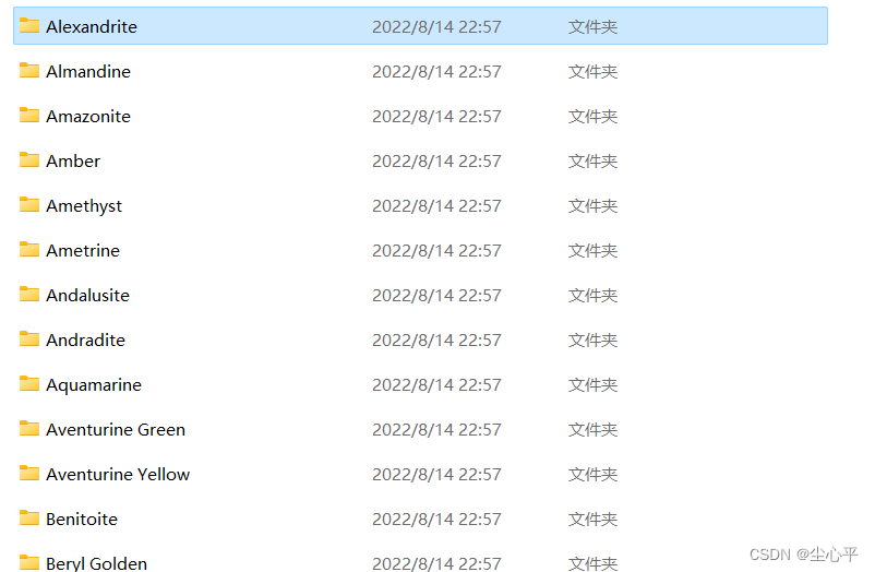
数据集采取文件夹名为标签名的形式，共有87种分类

​数据集导入

采用 keras.preprocessing.image.image_dataset_from_directory 方法导入数据集

这里由于子目录太多，采用 os.listdir 获取子目录列表即标签列表

• 设置路径

  设置路径(\换/)  采用os.listdir设置标签 设置图片大小

train_dir = "E:/Download/data_set/Gemstones/train"
test_dir = "E:/Download/data_set/Gemstones/test"
class_names = os.listdir(train_dir)  # 通过os.listdir获取标签列表
image_width = 128
image_height = 128

• 导入训练集

因为训练集已分好,这里不再设置函数的subset和validation_split,直接读取即可

train_data = keras.preprocessing.image.image_dataset_from_directory(
    directory=train_dir,
    class_names=class_names,
    image_size=(image_height, image_width),
    seed=123
)

• 导入测试集

因为测试集已分好,这里同训练集一样,不再设置subset和validation_split

test_data = keras.preprocessing.image.image_dataset_from_directory(
    directory=test_dir,
    class_names=class_names,
    image_size=(image_height, image_width),
    seed=123
)

• 设置预取加快训练速度

采用cache()和prefetch()函数预取

train_data = train_data.cache().shuffle(1000).prefetch(tf.data.AUTOTUNE)
test_data = test_data.cache().prefetch(tf.data.AUTOTUNE)

构建CNN网络模型

这里采用models.Sequential构建网络模型,且由于过拟合,采用正则化和Dropout

model = models.Sequential([
    layers.Rescaling(1 / 255.0, input_shape=(image_height, image_width, 3)),

    layers.Conv2D(128, (3, 3), padding="same", activation="relu",kernel_regularizer=keras.regularizers.L1L2(0.03)),
    layers.MaxPooling2D(),

    layers.Conv2D(128, (3, 3), activation="relu", padding="same"),
    layers.MaxPooling2D(),

    layers.Conv2D(256, (3, 3), activation="relu", padding="same"),
    layers.MaxPooling2D(),

    layers.Flatten(),
    layers.Dropout(0.6),
    layers.Dense(256, activation="relu"),
    layers.Dense(87)
])

编译运行神经网络

# 编译训练网络模型
model.compile(optimizer="adam",
              loss=tf.keras.losses.SparseCategoricalCrossentropy(from_logits=True),
              metrics=['accuracy'])

history = model.fit(train_data, validation_data=test_data, epochs=10)

评估模型

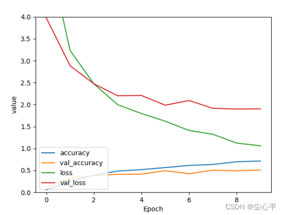
# 输出网络模型loss、val_loss变化曲线
plt.plot(history.history['accuracy'], label='accuracy')  # 训练集准确度
plt.plot(history.history['val_accuracy'], label='val_accuracy ')  # 验证集准确度
plt.plot(history.history['loss'], label='loss')  # 训练集损失程度
plt.plot(history.history['val_loss'], label='val_loss')  # 验证集损失程度
plt.xlabel('Epoch')  # 训练轮数
plt.ylabel('value')  # 值
plt.ylim([0,4])
plt.legend(loc='lower left')  # 图例位置
plt.show()

预测测试集

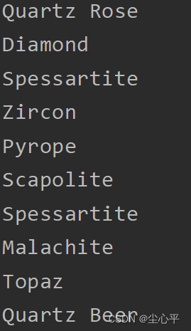
# 预测
pre = model.predict(test_data)
for i in range(20):
    print(pre[i])
for i in range(20):
    print(class_names[numpy.array(pre[i]).argmax()])
# 绘画数据集图像，查看导入是否完成
plt.figure(figsize=(20, 10))
for test_image, test_label in test_data.take(1):
    for i in range(20):
        plt.subplot(5, 10, i + 1)
        plt.xticks([])
        plt.yticks([])
        plt.grid(False)
        plt.imshow(test_image[i].numpy().astype('uint8') / 255.0, cmap=plt.cm.binary)
        plt.xlabel(class_names[test_label[i]])
    plt.show()

 这里预测测试集前20个

 正确率大概只有0.5很不理想,后续仍要改进

保存模型

这里采用SavedModel方法保存模型

save_path = "net/Gemstones"
model.save(save_path)