python学习——pandas数据处理 & 时间序列案例 & matplotlib绘图案例

---

pandas数据处理

1.合并数据

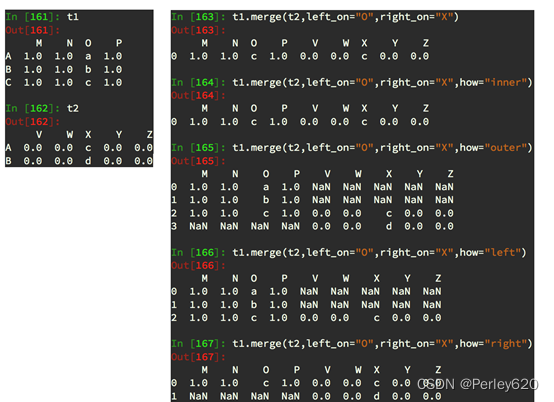
merge:按照指定的列把数据按照一定的方式合并到一起
默认的合并方式inner，交集
merge outer，并集，NaN补全
merge left，左边为准，NaN补全
merge right，右边为准，NaN补全

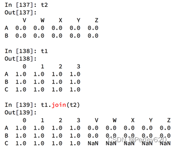
1) 堆叠合并

#内连inner返回索引重叠部分，外连outer返回返回并集数据
#1行对齐，0列对齐
pd.concat([df1,df2],axis=1,join='inner')
pd.concat([df1,df2],axis=1,join='outer')
pd.concat([df3,df4],axis=0,join='inner')
df3.append(df4) #纵向堆叠，列名必须一致

2) 主键合并

pd.merge(detail1,order,left_on='order_id',right_on = 'info_id')
data1=pd.merge(prior,products,on=["product_id","product_id"])
order.rename({
    
    'info_id':'order_id'},inplace=True) #换名字
detail1.join(order,on='order_id',rsuffix='1') #主键名必须一样

3) 重叠合并

dict2 = {
    
    'ID':[1,2,3,4,5,6,7,8,9],
         'System':[np.nan,np.nan,'win7',np.nan,
                'win8','win7',np.nan,np.nan,np.nan],
        'cpu':[np.nan,np.nan,'i3',np.nan,'i7',
                'i5',np.nan,np.nan,np.nan]}
## 转换两个字典为DataFrame
df5 = pd.DataFrame(dict1)
df6 = pd.DataFrame(dict2)
df5.combine_first(df6) #两表数据一一比较，完整表格内容

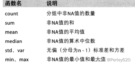
2.分组和聚合

grouped = df.groupby(by=“columns_name”)
grouped是一个DataFrameGroupBy对象，是可迭代的
grouped中的每一个元素是一个元组
元组里面是（索引(分组的值)，分组之后的DataFrame）

import pandas as pd
import numpy as np
file_path = "./starbucks_store_worldwide.csv"
df = pd.read_csv(file_path)
print(df.head(1))
print(df.info())
grouped = df.groupby(by="Country")
# print(grouped)

#DataFrameGroupBy
#可以进行遍历
for i,j in grouped:
    print(i)
    print("-"*100)
    print(j,type(j))
    print("*"*100)
df[df["Country"]=="US"]
#调用聚合方法,统计求和

country_count = grouped["Brand"].count()
print(country_count["US"])
print(country_count["CN"])

#统计中国每个省店铺的数量
china_data = df[df["Country"] =="CN"]
grouped = china_data.groupby(by="State/Province").count()["Brand"]
print(grouped)

#数据按照多个条件进行分组,返回Series
grouped = df["Brand"].groupby(by=[df["Country"],df["State/Province"]]).count()
print(grouped)
print(type(grouped))

#数据按照多个条件进行分组,返回DataFrame
grouped1 = df[["Brand"]].groupby(by=[df["Country"],df["State/Province"]]).count()
# grouped2= df.groupby(by=[df["Country"],df["State/Province"]])[["Brand"]].count()
# grouped3 = df.groupby(by=[df["Country"],df["State/Province"]]).count()[["Brand"]]

print(grouped1,type(grouped1))
# print("*"*100)
# print(grouped2,type(grouped2))
# print("*"*100)
# print(grouped3,type(grouped3))

#索引的方法和属性
print(grouped1.index)

3.索引和符合索引

简单的索引操作：
• 获取index：df.index
• 指定index ：df.index = [‘x’,‘y’]
• 重新设置index : df.reindex(list(“abcedf”))
• 指定某一列作为index ：df.set_index(“Country”,drop=False)
• 返回index的唯一值：df.set_index(“Country”).index.unique()
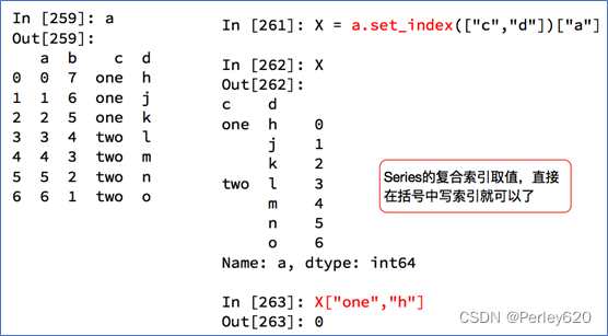
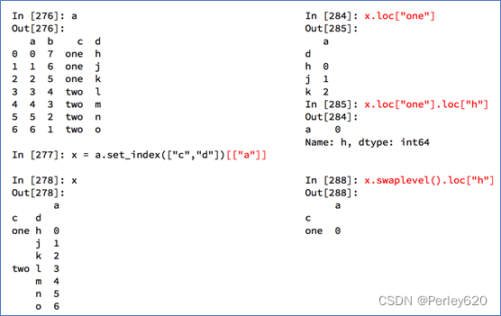
• a.set_index([“c”,“d”])即设置两个索引

Series复合索引

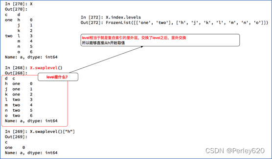
DataFrame复合索引

4.去除重复值

detail['dishes_name'].drop_duplicates()#去重全部列
detail.drop_duplicates(subset = ['order_id','emp_id']) #去重某些列

5.处理缺失值

对于NaN的数据，在numpy中我们是如何处理的？
在pandas中我们处理起来非常容易

判断数据是否为NaN：pd.isnull(df),pd.notnull(df)

处理方式1：删除NaN所在的行列t.dropna (axis=0, how=‘any’, inplace=False)
处理方式2：填充数据，t.fillna(t.mean()),t.fiallna(t.median()),t.fillna(0)

处理为0的数据：t[t==0]=np.nan
当然并不是每次为0的数据都需要处理
计算平均值等情况，nan是不参与计算的，但是0会

detail.isnull().sum()   #特征缺失的数目
detail.notnull().sum()  #特征非缺失的数目
detail.dropna(axis = 1,how ='any') #去除缺失的列
detail = detail.fillna(-99)        #替换缺失值

from scipy.interpolate import interp1d
LinearInsValue1 = interp1d(x,y1,kind='linear') ##线性插值拟合x,y1
print('当x为6、7时，使用线性插值y1为：',LinearInsValue1([6,7]))

LargeInsValue1 = lagrange(x,y1) ##拉格朗日插值拟合x,y1
SplineInsValue1 = spline(x,y1,xnew=np.array([6,7]))

6.处理离群值

import matplotlib.pyplot as plt
plt.figure(figsize=(10,8)) 
p = plt.boxplot(detail['counts'].values,notch=True)   ##画出箱线图
outlier1 = p['fliers'][0].get_ydata()   ##fliers为异常值的标签
plt.savefig('../tmp/菜品异常数据识别.png')
plt.show()

## 定义拉依达准则识别异常值函数
def outRange(Ser1):
    boolInd = (Ser1.mean()-3*Ser1.std()>Ser1) | \
    (Ser1.mean()+3*Ser1.var()< Ser1)
    index = np.arange(Ser1.shape[0])[boolInd]
    outrange = Ser1.iloc[index]
    return outrange
outlier = outRange(detail['counts'])
print('使用3o原则拉依达准则判定异常值个数为:',outlier.shape[0])
print('异常值的最大值为：',outlier.max())
print('异常值的最小值为：',outlier.min())

7.标准化数据

1) 离差标准化函数

## 自定义离差标准化函数
def MinMaxScale(data):
    data=(data-data.min())/(data.max()-data.min())
    return data
##对菜品订单表售价和销量做离差标准化
data1=MinMaxScale(detail['counts'])

2) 标准差标准化函数

##自定义标准差标准化函数
def StandardScaler(data):
    data=(data-data.mean())/data.std()
    return data
##对菜品订单表售价和销量做标准化
data4=StandardScaler(detail['counts'])

3) 小数定标差标准化函数

##自定义小数定标差标准化函数
def DecimalScaler(data):
    data=data/10**np.ceil(np.log10(data.abs().max()))
    return data
##对菜品订单表售价和销量做标准化
data7=DecimalScaler(detail['counts'])

8.转换数据–离散处理

##哑变处理（非数值型数据处理）
pd.get_dummies(data)

##等宽法离散
price = pd.cut(detail['amounts'],5)
##自定义等频法离散化函数
def SameRateCut(data,k):
    w=data.quantile(np.arange(0,1+1.0/k,1.0/k))
    data=pd.cut(data,w)
    return data
result=SameRateCut(detail['amounts'],5).value_counts() #售价等频法离散化
#自定义数据k-Means聚类离散化函数
def KmeanCut(data,k):
    from sklearn.cluster import KMeans #引入KMeans
    kmodel=KMeans(n_clusters=k)   #建立模型
    kmodel.fit(data.values.reshape((len(data), 1)))    #训练模型
    c=pd.DataFrame(kmodel.cluster_centers_).sort_values(0) #输出聚类中心并排序
    w=c.rolling(2).mean().iloc[1:]    #相邻两项求中点，作为边界点
    w=[0]+list(w[0])+[data.max()]    #把首末边界点加上
    data=pd.cut(data,w)
    return data
#菜品售价等频法离散化
result=KmeanCut(detail['amounts'],5).value_counts()

9.时间序列

Lat，lng：经纬度

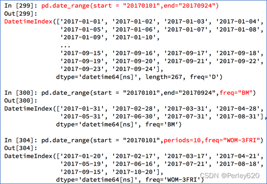
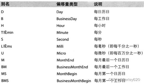
pd.date_range(start=None, end=None, periods=None, freq=‘10D’)#十天
start和end以及freq配合能够生成start和end范围内以频率freq的一组时间索引
start和periods以及freq配合能够生成从start开始的频率为freq的periods个时间索引

时间字符串转换成时间序列

index=pd.date_range(“20170101”,periods=10)
df = pd.DataFrame(np.random.rand(10),index=index)

回到最开始的911数据的案例中，我们可以使用pandas提供的方法把时间字符串转化为时间序列

df[“timeStamp”] = pd.to_datetime(df[“timeStamp”],format=“”)
format参数大部分情况下可以不用写，但是对于pandas无法格式化的时间字符串，我们可以使用该参数，比如包含中文

重采样

重采样：指的是将时间序列从一个频率转化为另一个频率进行处理的过程，将高频率数据转化为低频率数据为降采样，低频率转化为高频率为升采样

pandas提供了一个resample的方法来帮助我们实现频率转化

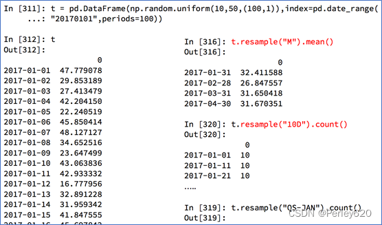
t=pd.DataFrame(np.random.uniform(10,50,(100,1)),index=pd.date_range("20170101",periods=100))
a=t.resample("10D").mean()
b=t.resample("QS-JAN").count()#每季度最后一月第一个日历日
print(b)

DatetimeIndex可以理解为时间戳
PeriodIndex可以理解为时间段

periods = pd.PeriodIndex(year=data["year"],month=data["month"],day=data["day"],hour=data["hour"],freq="H")

那么如果给这个时间段降采样呢？

data = df.set_index(periods).resample("10D").mean()

【案例】时间序列案例

显示中文，输出大列表处理

plt.rcParams['font.sans-serif'] = 'SimHei'
plt.rcParams['axes.unicode_minus'] = False ## 设置正常显示符号
# 设置显示的最大列、宽等参数，消掉打印不完全中间的省略号
# pd.set_option('display.max_columns', 1000)
pd.set_option('display.width', 1000)#加了这一行那表格的一行就不会分段出现了
# pd.set_option('display.max_colwidth', 1000)
# pd.set_option('display.height', 1000)
#显示所有列
pd.set_option('display.max_columns', None)
#显示所有行
pd.set_option('display.max_rows', None)

案例1：911的紧急电话的数据

现在我们有2015到2017年25万条911的紧急电话的数据，请统计出出这些数据中不同类型的紧急情况的次数，如果我们还想统计出不同月份不同类型紧急电话的次数的变化情况，应该怎么做呢？

1）请统计出出这些数据中不同类型的紧急情况的次数

我的方法：用时太长

import pandas as pd
import matplotlib.pyplot as plt
import numpy as np
file_path = "./911.csv"
df = pd.read_csv(file_path)
# print(df.info())
# print(df.head(10))

#字符串转换成列表，取第一个字符串
a=df["title"].str.split(":").tolist()
type_list=[i[0] for i in a]
# print(type_list)

temp_list = type_list
genre_list = list(set(type_list))

#构造全为0的数组
zeros_df = pd.DataFrame(np.zeros((df.shape[0],len(genre_list))),columns=genre_list)

#给每个电影出现分类的位置赋值1
for i in range(df.shape[0]):
    #zeros_df.loc[0,["Sci-fi","Mucical"]] = 1
    zeros_df.loc[i,temp_list[i]] = 1

#统计每个分类的电影的数量和
genre_count = zeros_df.sum(axis=0)
print(genre_count)

#排序
genre_count = genre_count.sort_values()
_x = genre_count.index
_y = genre_count.values
#画图
plt.figure(figsize=(20,8),dpi=80)
plt.bar(range(len(_x)),_y,width=0.4,color="orange")
plt.xticks(range(len(_x)),_x)
plt.show()

方法2：遍历次数减少，布尔索引赋值

# coding=utf-8
import pandas as pd
import numpy as np
from matplotlib import pyplot as plt

df = pd.read_csv("./911.csv")

print(df.head(5))
#获取分类
# print()df["title"].str.split(": ")
temp_list = df["title"].str.split(": ").tolist()
cate_list = list(set([i[0] for i in temp_list]))
print(cate_list)

#构造全为0的数组
zeros_df = pd.DataFrame(np.zeros((df.shape[0],len(cate_list))),columns=cate_list)

#赋值
for cate in cate_list:
    zeros_df[cate][df["title"].str.contains(cate)] = 1
    # break
# print(zeros_df)

sum_ret = zeros_df.sum(axis=0)
print(sum_ret)

方法3：添加一列，按照该列进行分组

# coding=utf-8
import pandas as pd
import numpy as np
from matplotlib import pyplot as plt

df = pd.read_csv("./911.csv")

print(df.head(5))
#获取分类
# print()df["title"].str.split(": ")
temp_list = df["title"].str.split(": ").tolist()
cate_list = [i[0] for i in temp_list]
df["cate"] = pd.DataFrame(np.array(cate_list).reshape((df.shape[0],1)))

# print(df.head(5))
print(df.groupby(by="cate").count()["title"])

2）不同月份不同类型 、不同月份电话次数

第二问

1. 统计出911数据中不同月份电话次数的变化情况
2. 统计出911数据中不同月份不同类型的电话的次数的变化情况

重新定义时间格式，时间那一列更改

import pandas as pd
import numpy as np
from matplotlib import pyplot as plt

df = pd.read_csv("./911.csv")
df["timeStamp"] = pd.to_datetime(df["timeStamp"])
df.set_index("timeStamp",inplace=True)#原地替换

#统计出911数据中不同月份电话次数的
count_by_month = df.resample("M").count()["title"]
print(count_by_month)

#画图
_x = count_by_month.index
_y = count_by_month.values

# for i in _x:
#     print(dir(i))
#     break
_x = [i.strftime("%Y%m%d") for i in _x] #重新定义时间的格式
plt.figure(figsize=(20,8),dpi=80)
plt.plot(range(len(_x)),_y)
plt.xticks(range(len(_x)),_x,rotation=45)
plt.show()

第二问我的

import pandas as pd
import matplotlib.pyplot as plt
import numpy as np

file_path = "./911.csv"
df = pd.read_csv(file_path)
# print(df.info())
df["timeStamp"] = pd.to_datetime(df["timeStamp"],format="")
temp_list = df["title"].str.split(": ").tolist()
cate_list = [i[0] for i in temp_list]
df["cate"] = pd.DataFrame(np.array(cate_list).reshape((df.shape[0],1)))

# print(df.info())

data_mon=df.set_index("timeStamp")
grouped=data_mon.groupby(by="cate")

plt.figure(figsize=(20,8),dpi=80)

for i,j in grouped:
    data1=j.resample("M").count()["title"]
    _x = data1.index
    _y = data1.values
    plt.plot(range(len(_x)),_y,label="i")
_x = [i.strftime("%Y%m%d") for i in _x] #重新定义时间的格式
plt.xticks(range(len(_x)),_x,rotation=45)
plt.show()

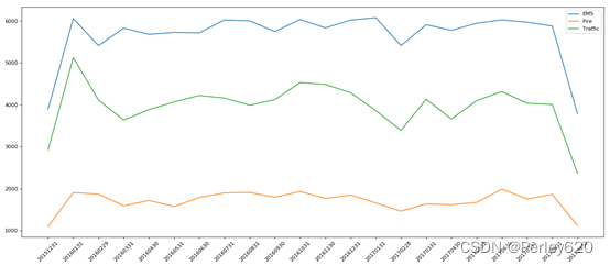
第二问 分组后的遍历画图Group

# coding=utf-8
#911数据中不同月份不同类型的电话的次数的变化情况
import pandas as pd
import numpy as np
from matplotlib import pyplot as plt

#把时间字符串转为时间类型设置为索引
df = pd.read_csv("./911.csv")
df["timeStamp"] = pd.to_datetime(df["timeStamp"])

#添加列，表示分类
temp_list = df["title"].str.split(": ").tolist()
cate_list = [i[0] for i in temp_list]
# print(np.array(cate_list).reshape((df.shape[0],1)))
df["cate"] = pd.DataFrame(np.array(cate_list).reshape((df.shape[0],1)))
df.set_index("timeStamp",inplace=True)
print(df.head(1))
plt.figure(figsize=(20, 8), dpi=80)

#分组
for group_name,group_data in df.groupby(by="cate"):
    #对不同的分类都进行绘图
    count_by_month = group_data.resample("M").count()["title"]
    # 画图
    _x = count_by_month.index
    print(_x)
    _y = count_by_month.values
    _x = [i.strftime("%Y%m%d") for i in _x]

    plt.plot(range(len(_x)), _y, label=group_name)
plt.xticks(range(len(_x)), _x, rotation=45)
plt.legend(loc="best")
plt.show()

案例2：空气质量数据

现在我们有北上广、深圳、和沈阳5个城市空气质量数据，请绘制出5个城市的PM2.5随时间的变化情况
观察这组数据中的时间结构，并不是字符串，这个时候我们应该怎么办？
数据来源： https://www.kaggle.com/uciml/pm25-data-for-five-chinese-cities
请绘制出5个城市的PM2.5随时间的变化情况

分开的时间数据处理，时间格式重新定义

# coding=utf-8
import pandas as pd
from matplotlib import  pyplot as plt
file_path = "./PM2.5/BeijingPM20100101_20151231.csv"

df = pd.read_csv(file_path)

#把分开的时间字符串通过periodIndex的方法转化为pandas的时间类型
period = pd.PeriodIndex(year=df["year"],month=df["month"],day=df["day"],hour=df["hour"],freq="H")
df["datetime"] = period
# print(df.head(10))

#把datetime 设置为索引
df.set_index("datetime",inplace=True)
#进行降采样
df = df.resample("7D").mean()
print(df.head())
#处理缺失数据，删除缺失数据
# print(df["PM_US Post"])

data  =df["PM_US Post"]
data_china = df["PM_Nongzhanguan"]
print(data_china.head(100))
#画图
_x = data.index
_x = [i.strftime("%Y%m%d") for i in _x]
_x_china = [i.strftime("%Y%m%d") for i in data_china.index]
print(len(_x_china),len(_x_china))
_y = data.values
_y_china = data_china.values

plt.figure(figsize=(20,8),dpi=80)
plt.plot(range(len(_x)),_y,label="US_POST",alpha=0.7)
plt.plot(range(len(_x_china)),_y_china,label="CN_POST",alpha=0.7)
plt.xticks(range(0,len(_x_china),10),list(_x_china)[::10],rotation=45)
plt.legend(loc="best")
plt.show()

案例3：简单的预测问题

缩小数据，选取部分数据；删除数据，分组后逆向操作；isin操作

# 读取数据
data = pd.read_csv("./data/FBlocation/train.csv")
# print(data.head(10))
# 处理数据
# 1、缩小数据,查询数据晒讯
data = data.query("x > 1.0 &  x < 1.25 & y > 2.5 & y < 2.75")
# 处理时间的数据
time_value = pd.to_datetime(data['time'], unit='s')
print(time_value)

# 把日期格式转换成 字典格式
time_value = pd.DatetimeIndex(time_value)
# 构造一些特征
data['day'] = time_value.day
data['hour'] = time_value.hour
data['weekday'] = time_value.weekday

# 把时间戳特征删除
data = data.drop(['time'], axis=1)#1表示列，0表示行
print(data)#没有时间戳特征的数据
# 把签到数量少于n个目标位置删除
place_count = data.groupby('place_id').count()
tf = place_count[place_count.row_id > 3].reset_index()#分组后逆操作，重新设置索引
data = data[data['place_id'].isin(tf.place_id)]
# 取出数据当中的特征值和目标值
y = data['place_id']#取目标值
x = data.drop(['place_id'], axis=1)#删除特征值就得到目标值

【案例】matplotlib绘图案例

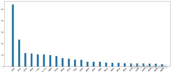
案例一：店铺总数排名前10的国家+中国每个城市的店铺数量

使用matplotlib呈现出店铺总数排名前10的国家
使用matplotlib呈现出中国每个城市的店铺数量

import pandas as pd
import matplotlib.pyplot as plt

file_path = "./starbucks_store_worldwide.csv"
df = pd.read_csv(file_path)

df1 = df[["Brand"]].groupby(by=[df["Country"]]).count()
genre_count1 = df1.sort_values(by="Brand",ascending=False)[:10]

_x = genre_count1.index
_y = genre_count1.iloc[:,0]

#画图
plt.figure(figsize=(20,8),dpi=80)
plt.bar(range(len(_x)),_y,width=0.4,color="orange")
plt.xticks(range(len(_x)),_x)
plt.show()

import pandas as pd
from matplotlib import pyplot as plt

file_path = "./starbucks_store_worldwide.csv"
df = pd.read_csv(file_path)

#使用matplotlib呈现出店铺总数排名前10的国家
#准备数据
data1 = df.groupby(by="Country").count()["Brand"].sort_values(ascending=False)[:10]

_x = data1.index
_y = data1.values

#画图
plt.figure(figsize=(20,8),dpi=80)
plt.bar(range(len(_x)),_y)
plt.xticks(range(len(_x)),_x)
plt.show()

import pandas as pd
import matplotlib.pyplot as plt
plt.rcParams['font.sans-serif'] = 'SimHei'
plt.rcParams['axes.unicode_minus'] = False ## 设置正常显示符号
pd.set_option('display.width', 1000)#加了这一行那表格的一行就不会分段出现了
pd.set_option('display.max_columns', None)
pd.set_option('display.max_rows', None)

file_path = "./starbucks_store_worldwide.csv"
df = pd.read_csv(file_path)
china_data = df[df["Country"] =="CN"]
grouped = china_data.groupby(by="City").count()["Brand"].sort_values(ascending=False)
print(grouped)

data1=grouped[:25]

_x = data1.index
_y = data1.values

#画图
plt.figure(figsize=(20,8),dpi=80)
plt.bar(range(len(_x)),_y,width=0.3)
plt.xticks(range(len(_x)),_x,rotation=45)
plt.show()

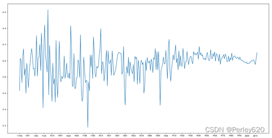
案例二：全球排名靠前的10000本书的数据

现在我们有全球排名靠前的10000本书的数据，那么请统计一下下面几个问题：

1. 不同年份书的数量
2. 不同年份书的平均评分情况

import pandas as pd
import matplotlib.pyplot as plt
plt.rcParams['font.sans-serif'] = 'SimHei'
plt.rcParams['axes.unicode_minus'] = False ## 设置正常显示符号
pd.set_option('display.width', 1000)#加了这一行那表格的一行就不会分段出现了
pd.set_option('display.max_columns', None)
pd.set_option('display.max_rows', None)

file_path = "books.csv"
df = pd.read_csv(file_path)
# print(df.info())
# print(df.head(1))
df1=df[pd.notnull(df["original_publication_year"])]#处理缺失值
book_year_num=df1.groupby(by="original_publication_year").count()["id"].sort_values(ascending=False)

#第二问：不同年份的书的平均评分
book_mean_rates=df1["average_rating"].groupby(by=df1["original_publication_year"]).mean()
#画图
plt.figure(figsize=(20,10),dpi=80)
_x=book_mean_rates.index
_y=book_mean_rates.values
plt.plot(range(len(_x)),_y)
plt.xticks(list(range(len(_x)))[::10],_x[::10].astype(int))#rotation旋转90度
plt.show()