Contour Detection and Hierarchical Image Segmentation

一 、论文原理分析

算法路线：gPb—->OWT—–>UCM

每一部分的功能：

• gPb（Global Pb）：计算每一个pixel作为boundary的可能性，即pixel的weight；
• OWT（Oriented Watershed Transform）将上述gPb的结果转换为多个闭合的regions；
• UCM（Ultrametric Contour Map）将上述regions集，转换为hierarchical tree。

这里出现了很多名词，如：什么是hierarchical tree？什么是Oriented Watershed Transform。

1.1 gPb（Global Probability of Boundary）

gPb是mPb和sPb的加权和。 
mPb是什么？sPb是什么？

- step1：计算G(x,y,θ) 
对于每一个pixel，以其为圆心，做一个圆形： 
 
用倾斜角为θ的直径，将圆形划分为两个区域，对于每一个区域中的pixels，做出它们的histogram，如下：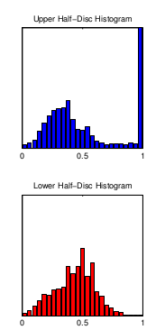 
 
使用histogram数据，计算其卡方距离：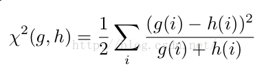 
 
该距离即为G(x,y,θ)，代表pixel(x,y)以θ为方向的gradient magnitude；

- step2：计算mPb 
普通的Pb算法，将一幅图片，分解为4个不同的feature channels，分别为brightness、color a、color b以及texture channel，其中前三个channels是基于CIE color space。

而每个pixel的weight就是由这4个channels下计算得到的G(x,y,θ)值的加权和。

针对普通的Pb算法，作者提出了multiscale的方法，即为mPb。

它的原理是在原有Pb算法的基础上，同时使用多个圆形直径长度δ（作者使用三个，[ δ/2 ,δ, 2δ]），针对每一个δ，计算其G（x，y，θ），最终公式如下：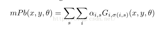 
 
公式中的i代表channel，s代表scale。 
意思是，对于每一个pixel，我们计算其在不同直径条件下的每一个feature channel的和，作为其mPb值。 
α代表每一个不同直径条件下的每一个feature channel的权重，是针对F-measure进行gradient ascent得到，使用的训练集是BSDS。

- step3：计算sPb 
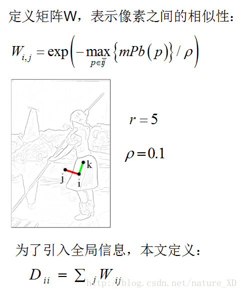
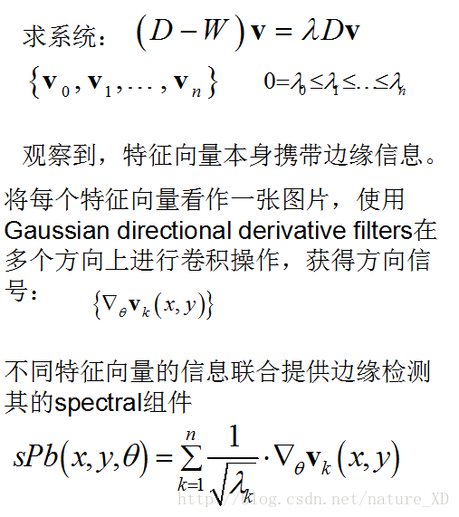
作者首先作出了一个sparse symmetric affinity matrix W，其中每一个元素Wij的计算如下：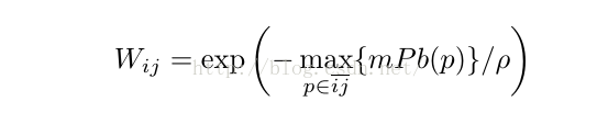 
 
i，j代表两个距离不超过半径r（单位：像素，作者在代码中设定r=5）的像素，p是两个像素连成的线段上的任意一个点，找到某两个pixel连成的线段上的pixel的weight的最大值。ρ是常数，作者代码中设定为ρ= 0.1。

扫描二维码关注公众号，回复： 152758 查看本文章

该矩阵W代表pixels之间的相似度，通过令：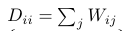 
 
得到矩阵D，由：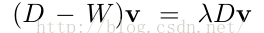 
 
计算得到前n+1个特征向量，代码中作者使用的是n=16.

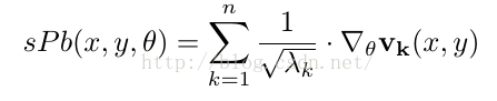
接着，作者将每一个特征向量视为一幅图片，使用Gaussian Directional Derivative Filters对其进行卷积操作，得到：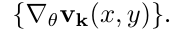 
 
从而得到sPb计算公式： 
 
其中的参数：是将特征向量的物理解释问题视为mass-spring system得到的。

- step4：计算gPb 
综合mPb和sPb，得到gPb。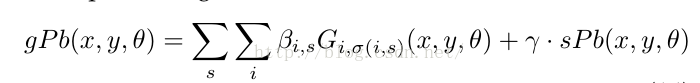 
 
β参数前面前文已经解释，参数γ是使用BSDS训练集，通过在 
F-measure = 
上进行gradient ascent得到。

最后，对于该gPb值进行sigmoid函数变换，使其值处于0-1之间，作为该pixel作为boundary的probability，我在下文都将其称为pixel的weight。

1.2 OWT（Oriented Watershed Transform）

对于每一个pixel，代入八个设定的角度θ∈[0, pi]，取其最大值作为边缘的权重。该E(x,y,θ)即为gPb公式。 
 
这样，每一个pixel均被赋予一个0到1之间的值，其值大小表示该pixel是boundary的可能性。

接着使用WT（Watershed Transform）技术，将以上的输入转化为一系列Po（regions）和Ko（arcs）。如图：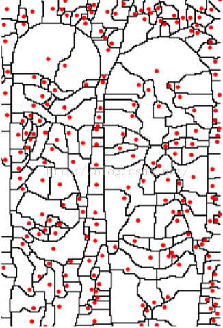 
 
图中，红点为其region的minimal，arcs为其边界。

原来的WT算法，是使用该arc上的pixels的weight的平均值作为其强度。

然而这种方法，会导致一些弱arc的某些pixels因为处于强arc的周边，在计算 的过程中，选择了针对强arc的方向θ，从而该pixel的值偏大，于是弱arc的强度也相应偏大。

此句话的意思为：计算某一个arc pixel的值时，有八个方向的权重可以选择，之前的选择方案是无论什么情况下均选择使得E(x,y,θ)最大的θ方向的值，而并没有考虑arc的走势，可能会导致本来值应该较小的元素，因为θ方向E(x,y,θ)值最大，取该方向后，导致计算出来的该像素点的值也偏大

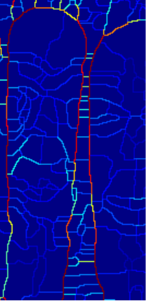
如下图所示，两个石头像的中间，有许多横的强arc：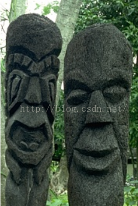 
  
原图中并没有这些横的强arc边缘，这是不合理的。

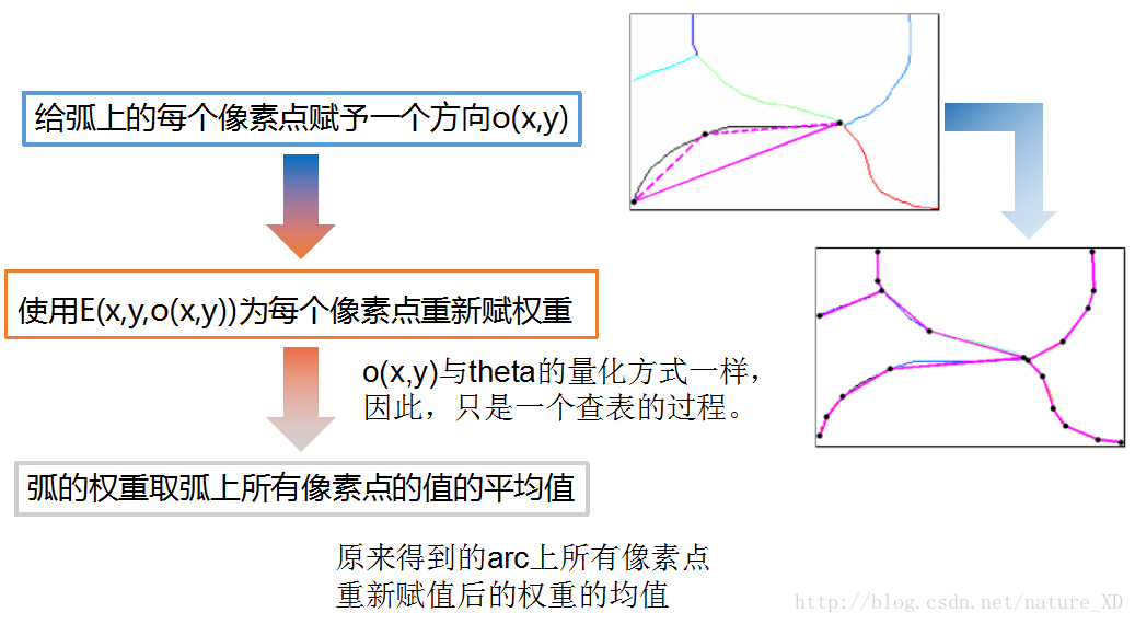
作者提出的OWT，是在原来WT的基础上，对所有处在arc上的pixel，重新选择合理的方向θ，计算E（x, y, θ），从而对arc的强度值作调整，方法如下：

这里对所有处在arc上的pixels重新选择方向，计算arc强度，那么如何判断哪些pixels处于arc上呢？使用原始WT计算一遍，得到哪些pixels属于regions，哪些pixels属于arcs，然后对于处于arc上的所有pixels重新计算其权值，计算方法为：选择沿着弧线方向的E（x, y, θ）得到E(x,y)；最后计算每个arc的强度，即arc上所有pixels的weight的平均值。

过程如下：

1. 对于每一个arc，将该arc subdivide（分割）为许多线段，如图： 
   
2. 计算每个线段的方向，使用o(x,y)表示其方向
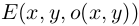
3. 使用下面的公式，重新计算每一个pixel的gPb（E(x,y)）值： 
   
4. 重新计算每个arc的强度，即取arc上所有pixels的weight的平均值作为arc最终的权重值。

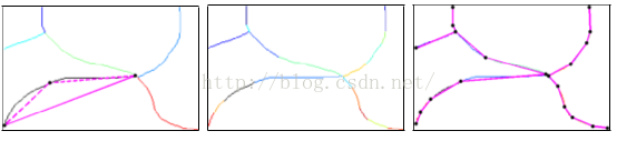
左为修改前，右为修改后：

 

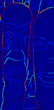
前面的内容总结为：使用四个通道特征（brightness、color a、color b and texture），三个半径尺寸，计算得到每个像素点在八个方向的权重，该权重大小指示该像素点为边界的可能性大小，即该点值某个方向的值越大，表示该点的为边界的可能性越大；取使得E(x,y,theta)最大的theta，得到gPb，即pixel(x,y)为边界的可能性E(x,y)，以得到的E(x,y)作为输入，使用WT将所有像素点分为Po（regions）和Ko（arcs），原来WT算法中arcs的权重直接采用该arc上所有pixels的权重的均值，现在重新计算arc上每个像素点沿arc方向的E(x,y,o(x,y))的值，然后再取arc上所有pixels的均值作为arc的值。

因为，如果不重新计算，直接取均值，有可能一条弧线上，一个权重较小的点，挨着一个权重较大的点，均值将使得该权重较小点的权重偏大。如图中横线，本来值较小，因为相交点沿红线方向的权重较大，如果相交点取沿红线方向的值，那么弧上点的值取平均的时候，该横线的整体权重被拉大。修改后，相交点，该点沿着红线方向的值较大，沿着横线方向的权重较小，所以横线的整体权重变得相对更加准确些。

为什么要计算一个像素点八个方向的权重？我觉得就是想要知道在哪个方向的时候，该像素点两边的差距最大，即边缘方向的问题，所以八个方向的计算是为了第二步，OWT的使用。 
WT，分水岭算法，使用E(x,y)作为其输入，将所有像素点分为Po（regions）和Ko（arcs），原来的arcs的权重直接采用该arc上所有pixels的权重的均值，现在重新计算arc上每个像素点沿arc方向的E(x,y,o(x,y))的值，然后再取arc上所有pixels的均值作为arc的值。

1.3 UCM（Ultrametric Contour Map）

为了在不同细节层次上对图像进行segmentation，作者使用了Ultrametric Contour Map（UCM）。

OWT算法已经output出细节度最高的regions集合，接下来，作者作出一个graph，如下：

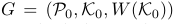
其中，Po是regions，Ko是arcs，W(Ko)是该arc的强度。该图以region作为node，若两region相邻，则其对应的两个node相连，连接强度为W(Ko);

下一步，设两两regions之间的dissimilarity为其共同arc的强度平均值。

使用一种基于graph的merging技术，以两两regions之间的dissimilarity作为衡量标准，将regions按照dissimilarity升序排列，依次将dissimilarity小的region合并，直到最后只有一个region，这样，就完成了hierarchical tree的建设。

Hierarchical Tree的构建过程，类似于Huffman树的构建过程

在这颗树中，因为生成树的每一个步骤，都是去除dissimilarity最小的arc，从而将两个region合并，因此，树中某个region元素的高度就代表着合并得到该region时，去除的arc的强度值大小，即：

H(R) = W(C)

• 1

因此，可以得到一个矩阵： 

该矩阵的元素代表细节度最高的segmentation下，所有regions两两之间的dissimilarity，其值由两region的最小公共所属region的高度 
 
决定。

元素值计算公式如下： 

总结：Hierarchical Tree 
Hierarchical Tree将OWT得到的结果，以regions为顶点，arc的强度为权重，使用graph的merging技术，类似于Huffman树的构建过程，每次从候选集中选择两个最小的node合并，本文即为每次从候选regions中选择两个拥有最小dissimilarity的regions，即两个最相近的regions。 
本文设两两regions之间的dissimilarity为其共同arc的强度平均值 
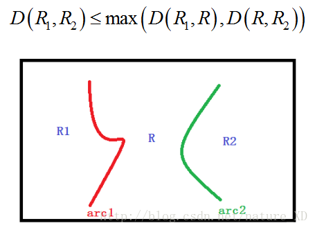
如果两个regions相邻，则其dissimilarity即为两个regions共同arc的强度；如果两个regions不相邻，则取其公共区域的高度，如下图所示：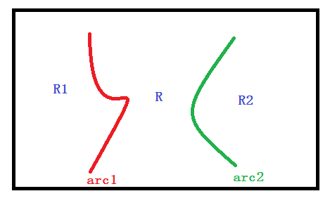 
 
设： 
D（R1，R）=avg（arc1） %R1和R的距离为两个regions公共弧的平均值 
D（R，R2）=avg（arc2） 
那么，D（R1，R2）= max（D（R1，R），D（R，R2）） 
因为，假设arc1的平均值小于arc2，即D（R1，R）< D（R，R2）,那么R和R1会先合并，设合并后的regions称为R3，那么R3与R2之间的dissimilarity即为arc2的平均值，因为R3和R2的公共弧为arc2。所以，R1和R2之间的dissimilarity如上。

对上面两个公式的计算仍然是不甚理解！！！

这是一个Ultrametric Contour Map（UCM）

因此，可以设定不同的阈值k，从而得到不同细节度的segmentation。

1.4 总结

作者在原有的方法上，主要做了这四个方面的革新：

1. 在contour detector部分中的mPb环节引入了multiscale的概念，提出了mPb算法，可以将其视作普通Pb算法的加强版，公式如下： 
   

2. 在contour detector部分中的sPb环节，对特征向量采取Gaussian directional derivative filters卷积操作，公式如下： 
   

3. 提出了OWT（Oriented Watershed Transform），对原来算法中受强boundary影响而存在问题的pixel，结合其所属arc的方向再次计算其weight。

4. 将OWT生成的region集合组合成UCM（Ultrametric Contour Map），使得我们可以通过阈值k来输出不同细节度的图像轮廓。

二、sPb的计算

 

---

OWT的思路来源

原始WT的说明： 

直接取arc上所有像素点的最大E(x,y)的均值的问题是：

原文： 
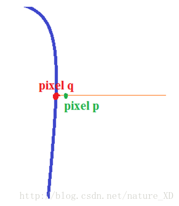
For example，a pixel could lie near but not on a strong vertical contour. If this pixel also happens to belong to a horizontal watershed arc, that arc would be errorneously upweighted.

我的理解： 
p到q是一个爬坡的过程，所以我们假设p点离q点足够近，那么p点使得E(x,y)最大的方向，很可能是沿着垂直方向的，而p在水平方向的权重可能不那么大，从而导致arc上整体权重偏大。

p点应取水平方向的E(x,y)，而不是垂直方向的！

---

UCM中的Ultrametric Property（超度量属性）

超度量空间，是一个将三角不等式替换为

d(x,z)<= max{d(x,y),d(y,z)}

• 1

的特殊度量空间。

构建的Hierarchical Tree满足超度量性质： 

因此，可以将得到的Hierarchy构建为UCM。

三、部分代码说明

如果需要分割效果图，运行BSR/grouping中代码，如果要看P-R曲线图就运行BSR/bench代码。

想要理解原理，最好下载源码。

在grouping中有文件夹：data、interactive、lib和source；文件example.m、run_bsds500.m 
data文件夹下：包含运行程序要输入的源文件和输出文件； 
lib文件夹：.m中使用addpath指令，将该目录下的文件加入到工作目录中，其下文件为使用mex编译过的C++文件或要使用的.m文件。 
source文件夹下：源文件，lib中某些文件是使用source中的源文件编译所得。 

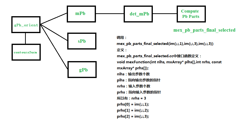
下面主要对该接口函数内部实现进行简要说明： 
接口函数的注释分为以下几个部分：

/*Compute bg histogram smoothing kernel*/
/*get_image*/
/*mirror border*/
/*convert to grayscale*/
/*gamma correct*/
/*convert to Lab*/
/*quantize color channels*/
/*compute texton filter set*/
/*compute textons*/
/*return textons*/
/*compute bg at each radius*/
/*compute cga at each radius*/
/*compute cgb at each radius*/
/*compute tg at each radius*/
/*return textons*/

• 1
• 2
• 3
• 4
• 5
• 6
• 7
• 8
• 9
• 10
• 11
• 12
• 13
• 14
• 15

分别对应程序运行中输出的内容为：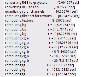 
 
lib_image命名空间下的函数，如 
lib_image::grayscale() 
lib_image类定义在： 
BSR/grouping/source/gpb_src/include/math/libraries/lib_image.hh中； 
相应的函数实现在 
BSR/grouping/source/gpb_src/src/math/libraries/lib_image.cc中。

其中的一些代码实现如下所示，代码布置比较容易看懂，作者将相关函数的实现集中在一起，并有较为详细的说明。

/*Image processing functions*/
class lib_image{
    public:

    /***********************************************
        **Image color space transforms.**
          -----------------------------
     Input RGB images should be scaled so that range 
     of possible values for each color channel is [0,1].
    ************************************************/
    /*Compute a grayscale image from an RGB image*/
    static matrix<> grayscale(
        const matrix<> &, /*r*/
        const matrix<> &, /*g*/
        const matrix<> & /*b*/
        );
    /*Normalize a grayscale image so that intensity values lie in [0,1]*/
    static void grayscale_normalize(matrix<> &);
    /*Normalize a grayscale image so that intensity values span the full [0,1] range*/
    static void grayscale_normalize_stretch(matrix<> &);

    /*Gamma correct the RGB image using the given correction value*/
    static void rgb_gamma_correct(
        matrix<>&, /*r*/
        matrix<>&, /*g*/
        matrix<>&, /*b*/
        double /*gamma*/
    );

    /*Normalize an Lab image so that values for each channel lie in [0,1]*/
    static void lab_normalize(
        matrix<>&,/*l*/
        matrix<>&,/*a*/
        matrix<>&/*b*/
    );

    /*Convert from RGB color space to XYZ color space*/
    static void rgb_to_xyz(
        matrix<>&, /*r (input) --> x(output)*/
        matrix<>&, /*g (input) --> y(output)*/
        matrix<>&  /*b (input) --> z(output)*/
    );

    /*Convert from RGB color space to Lab color space*/
    static void rgb_to_lab(
        matrix<>&, /*r (input) --> l(output)*/
        matrix<>&, /*g (input) --> a(output)*/
        matrix<>&  /*b (input) --> b(output)*/
    );
    ......

    /*  **用到的几个函数解析.** */

    /***********************************************
        **Gaussian Kernels.**
          -----------------------------
    The kernels are evaluated at integer coordinates in the range[-s,s] (in the 1D case) or 
    [-s_x,s_x]*[-s_y,s_y](in the 2D case), where s is the specified support.
    ************************************************/
    //一维的情形
    /* The length of the returned vector is 2*support + 1
    the support defaults to 3*sigma.
    The kernel is normalized to have unit L1 norm.
    */
    static matrix<> gaussian(
        double = 1, /*sigma*/
        unsigned int =0, /*derivative(0,1,2)*/
        bool = false /*take hilbert transform?*/
    );
    static matrix<> gaussian(
        double, /*sigma*/
        unsigned int , /*derivative(0,1,2)*/
        bool,  /*take hilbert transform?*/
        unsigned long /*support*/
    );
    //二维的情形
    static matrix gaussian_2D(
        double =1, /*sigma x*/
        double =1, /*sigma y*/
        double =0, /*orientation*/
        unsigned int =0, /*derivation in y-direction(0,1 or 2)*/
        bool =false /*take hilbert transform in y-direction?*/
    );
    static matrix gaussian_2D(
        double , /*sigma x*/
        double , /*sigma y*/
        double , /*orientation*/
        unsigned int; /*derivation in y-direction(0,1 or 2)*/
        bool , /*take hilbert transform in y-direction?*/
        unsigned long, /*x support*/
        unsigned long /*y support*/
    );
    /***********************************************
    Quantize image values into uniformly spaced bins in [0,1].
    Return the assignments and (optionally) bin centroids.
    ************************************************/
    static matrix<unsigned long> quantize_values(
        const matrix<>&,   /*image*/
        unsigned long      /* number of bins */ 
    );
    /***********************************************
        **Difference of histogram(2D).**
          -----------------------------

    ************************************************/
}

• 1
• 2
• 3
• 4
• 5
• 6
• 7
• 8
• 9
• 10
• 11
• 12
• 13
• 14
• 15
• 16
• 17
• 18
• 19
• 20
• 21
• 22
• 23
• 24
• 25
• 26
• 27
• 28
• 29
• 30
• 31
• 32
• 33
• 34
• 35
• 36
• 37
• 38
• 39
• 40
• 41
• 42
• 43
• 44
• 45
• 46
• 47
• 48
• 49
• 50
• 51
• 52
• 53
• 54
• 55
• 56
• 57
• 58
• 59
• 60
• 61
• 62
• 63
• 64
• 65
• 66
• 67
• 68
• 69
• 70
• 71
• 72
• 73
• 74
• 75
• 76
• 77
• 78
• 79
• 80
• 81
• 82
• 83
• 84
• 85
• 86
• 87
• 88
• 89
• 90
• 91
• 92
• 93
• 94
• 95
• 96
• 97
• 98
• 99
• 100
• 101
• 102
• 103
• 104
• 105
• 106

auto_collection< matrix<>, array_list< matrix<> > > lib_image::hist_gradient_2D(
   const matrix<unsigned long>&                 labels,
   unsigned long                                r,
   unsigned long                                n_ori,
   const matrix<>&                              smoothing_kernel,
   const distanceable_functor<matrix<>,double>& f_dist)
{
   /* construct weight matrix for circular disc */
   matrix<> weights = weight_matrix_disc(r);
   /* compute oriented gradient histograms */
   return lib_image::hist_gradient_2D(
      labels, weights, n_ori, smoothing_kernel, f_dist
   );
}

/*
 * Construct weight matrix for circular disc of the given radius.
 */
matrix<> weight_matrix_disc(unsigned long r) {
   /* initialize matrix */
   unsigned long size = 2*r + 1;
   matrix<> weights(size, size);
   /* set values in disc to 1 */
   long radius = static_cast<long>(r);
   long r_sq = radius * radius;
   unsigned long ind = 0;
   for (long x = -radius; x <= radius; x++) {
      long x_sq = x * x;
      for (long y = -radius; y <= radius; y++) {
         /* check if index is within disc */
         long y_sq = y * y;
         if ((x_sq + y_sq) <= r_sq)
            weights[ind] = 1;
         /* increment linear index */
         ind++;
      }
   }
   return weights;
}

• 1
• 2
• 3
• 4
• 5
• 6
• 7
• 8
• 9
• 10
• 11
• 12
• 13
• 14
• 15
• 16
• 17
• 18
• 19
• 20
• 21
• 22
• 23
• 24
• 25
• 26
• 27
• 28
• 29
• 30
• 31
• 32
• 33
• 34
• 35
• 36
• 37
• 38
• 39
• 40

参考文献

1、作者公布文章和资源下载地址为： 
http://www.eecs.berkeley.edu/Research/Projects/CS/vision/grouping/resources.html 
2、 Contour Detection and Hierarchical Image Segmentation 源码编译运行 
http://blog.csdn.net/blitzskies/article/details/19686179 
其中包括连接，对bench的测试，即P-R曲线的测试。 
3、Contour Detection and Hierarchical Image Segmentation 伯克利的一篇图像分割论文理解与学习 
http://blog.csdn.net/alex_luodazhi/article/details/47337327

4、https://blog.csdn.net/nature_XD/article/details/53375344?locationNum=9&fps=1