参考路径:目标检测RCNN系列的候选区选择算法——selective search(原理+Python实现)_macan_dct的博客-CSDN博客
作用:实际上就是在原图尽可能快,尽可能好的生成框选目标的候选框,避免使用穷举法导致的计算量过大的问题
策略: 遍历所有的尺度,但不同于暴力穷举,首先得到小尺度的候选区域,然后一次次合并得到大的候选区域
方案: 解决纹理问题使用,使用颜色特征;解决颜色特征不行的问题,使用纹理特征;解决尺度问题,使用候选区域的面积和互补性
具体操作思想大致如下:
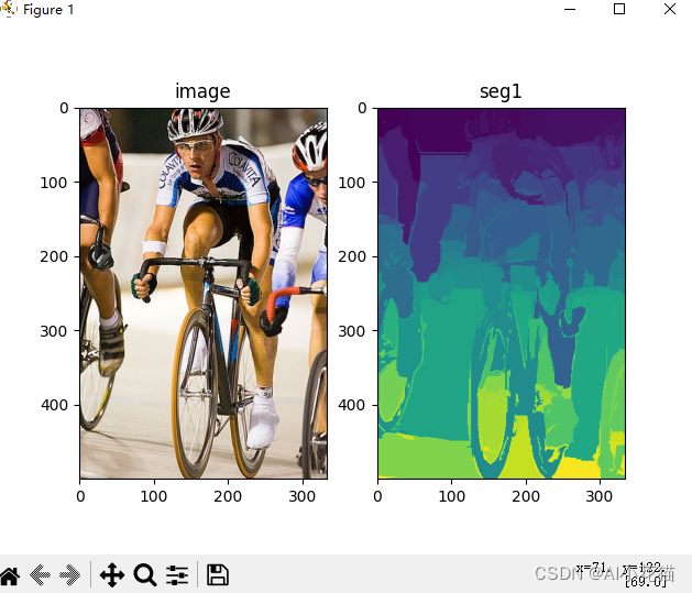
(1)selective search首先使用 Felzenswalb图像分割算法将图像分割成多个不同的块,每一个块代表分割算法得到的一个类,根据每个块的横纵坐标的最大值和最小值来初步产生一个候选区
import cv2
import numpy as np
from skimage import io as sio
from skimage.segmentation import felzenszwalb
import matplotlib.pyplot as plt

if __name__ == '__main__':
    sigma = 0.9
    kernel = 3
    K, min_size = 500, 10
    image = sio.imread(r"D:\personal\model_and_code\dataset\VOCdevkit\VOC2012\JPEGImages\2007_000129.jpg")
    # skimage自带的felzenszwalb算法
    seg1 = felzenszwalb(image, scale=K, sigma=sigma, min_size=min_size)

    fig = plt.figure()
    a = fig.add_subplot(121)
    plt.imshow(image)
    a.set_title("image")

    a = fig.add_subplot(122)
    plt.imshow(seg1)
    a.set_title("seg1")
    plt.show()
分割得到的每一类分割结果都会有像素位置的横坐标的左侧最小值min_x、纵坐标的左侧最小值min_y、横坐标的右侧最大值max_x、纵坐标的右侧最大值max_y,即[min_x, min_y, max_x, max_y]作为当前分割结果的候选区(框)
# pass 1: 根据分割类别,找到分割结果的每个类别像素位置的左上坐标和右下坐标
    for y, i in enumerate(img):
        for x, (r, g, b, l) in enumerate(i):
            # initialize a new region
            if l not in R:
                R[l] = {


                    "min_x": 0xffff, "min_y": 0xffff,
                    "max_x": 0,      "max_y": 0, "labels": [l]}
            # bounding box
            if R[l]["min_x"] > x:
                R[l]["min_x"] = x
            if R[l]["min_y"] > y:
                R[l]["min_y"] = y
            if R[l]["max_x"] < x:
                R[l]["max_x"] = x
            if R[l]["max_y"] < y:
                R[l]["max_y"] = y
(2)分割结果使用局部梯度算法(LBP)得到梯度信息,统计梯度直方图
# pass 2: 计算RGB空间下的梯度信息
tex_grad = _calc_texture_gradient(img)

def _calc_texture_gradient(img):
    """
        calculate texture gradient for entire image

        The original SelectiveSearch algorithm proposed Gaussian derivative
        for 8 orientations, but we use LBP instead.

        output will be [height(*)][width(*)]
    """
    ret = numpy.zeros((img.shape[0], img.shape[1], img.shape[2]))
    for colour_channel in (0, 1, 2):
        ret[:, :, colour_channel] = skimage.feature.local_binary_pattern(img[:, :, colour_channel], 8, 1.0)
    return ret
获取整张图像的梯度信息后,按照分割算法得到的像素级的分类结果,按照像素的类别计算同类下的梯度直方图
# texture histogram
R[k]["hist_t"] = _calc_texture_hist(tex_grad[:, :][img[:, :, 3] == k])

def _calc_texture_hist(img):
    BINS = 10
    hist = numpy.array([])
    for colour_channel in (0, 1, 2):
        # mask by the colour channel
        fd = img[:, colour_channel]
        # calculate histogram for each orientation and concatenate them all
        # and join to the result
        hist = numpy.concatenate([hist] + [numpy.histogram(fd, BINS, (0.0, 1.0))[0]])
    # L1 Normalize
    hist = hist / len(img)
    return hist
(3)分割结果为RGB空间,转成HSV空间,计算HSV空间下的颜色直方图
获取分割结果的HSV空间,然后按照通道计算颜色直方图,并进行归一化
# RGB空间转成HSV空间
hsv = skimage.color.rgb2hsv(img[:, :, :3])

def _calc_colour_hist(img):
    BINS = 25
    hist = numpy.array([])
    for colour_channel in (0, 1, 2):
        # extracting one colour channel
        c = img[:, colour_channel]
        # calculate histogram for each colour and join to the result
        hist = numpy.concatenate(
            [hist] + [numpy.histogram(c, BINS, (0.0, 255.0))[0]])
    # L1 normalize
    hist = hist / len(img)
    return hist
(4)分别根据颜色直方图和梯度直方图计算分割得到的那些发生重叠的候选区的颜色相似性和梯度相似性,还包括面积相似性、互补相似性
# extract neighbouring information
neighbours = _extract_neighbours(R)

# calculate initial similarities
S = {

    }
for (ai, ar), (bi, br) in neighbours:
    S[(ai, bi)] = _calc_sim(ar, br, imsize)


def _extract_neighbours(regions):

    def intersect(a, b):
        if (a["min_x"] < b["min_x"] < a["max_x"]
                and a["min_y"] < b["min_y"] < a["max_y"]) or (
            a["min_x"] < b["max_x"] < a["max_x"]
                and a["min_y"] < b["max_y"] < a["max_y"]) or (
            a["min_x"] < b["min_x"] < a["max_x"]
                and a["min_y"] < b["max_y"] < a["max_y"]) or (
            a["min_x"] < b["max_x"] < a["max_x"]
                and a["min_y"] < b["min_y"] < a["max_y"]):
            return True
        return False

    R = list(regions.items())
    neighbours = []
    for cur, a in enumerate(R[:-1]):
        for b in R[cur + 1:]:
            if intersect(a[1], b[1]):
                neighbours.append((a, b))

    return neighbours
(5)根据相似性合并这些重叠的候选区
首先,获取最大的相似度下标,
其次,获取候选区域最大类别数+1
然后,合并最大相似度的两个区域
然后,找到需要删除的含有i,j的keys
然后,重新计算两个区域之间的相似度
最后,获取最终的候选区域的rect,size,labels的结果值
# hierarchal search
while S != {

    }:

    # get highest similarity
    i, j = sorted(S.items(), key=lambda i: i[1])[-1][0]

    # merge corresponding regions
    t = max(R.keys()) + 1.0
    R[t] = _merge_regions(R[i], R[j])

    # mark similarities for regions to be removed
    key_to_delete = []
    for k, v in S.items():
        if (i in k) or (j in k):
            key_to_delete.append(k)

    # remove old similarities of related regions
    for k in key_to_delete:
        del S[k]

    # calculate similarity set with the new region
    for k in filter(lambda a: a != (i, j), key_to_delete):
        n = k[1] if k[0] in (i, j) else k[0]
        S[(t, n)] = _calc_sim(R[t], R[n], imsize)

regions = []
for k, r in R.items():
    regions.append({


        'rect': (
            r['min_x'], r['min_y'],
            r['max_x'] - r['min_x'], r['max_y'] - r['min_y']),
        'size': r['size'],
        'labels': r['labels']
    })
(6)计算候选区与ground truth的IOU,小于阈值的作为负样本,大于阈值的将真实类别作为其标签
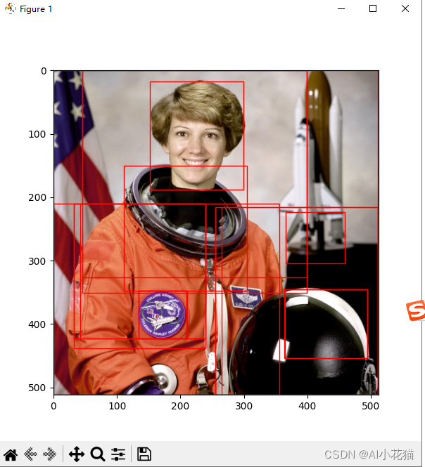
selective serach使用方法:
使用 pip install selectivesearch安装相应的库
from __future__ import (
    division,
    print_function,
)
import skimage.data
import matplotlib.pyplot as plt
import matplotlib.patches as mpatches
import selectivesearch


def main():
    # loading astronaut image
    img = skimage.data.astronaut()

    # perform selective search
    img_lbl, regions = selectivesearch.selective_search(
        img, scale=500, sigma=0.9, min_size=10)

    candidates = set()
    for r in regions:
        # excluding same rectangle (with different segments)
        if r['rect'] in candidates:
            continue
        # excluding regions smaller than 2000 pixels
        if r['size'] < 2000:
            continue
        # distorted rects
        x, y, w, h = r['rect']
        if w / h > 1.2 or h / w > 1.2:
            continue
        candidates.add(r['rect'])

    # draw rectangles on the original image
    fig, ax = plt.subplots(ncols=1, nrows=1, figsize=(6, 6))
    ax.imshow(img)
    for x, y, w, h in candidates:
        print(x, y, w, h)
        rect = mpatches.Rectangle(
            (x, y), w, h, fill=False, edgecolor='red', linewidth=1)
        ax.add_patch(rect)

    plt.show()


if __name__ == "__main__":
    main()
使用上述代码生成的候选区域绘制在图上如下所示: