全面详解gumbel softmax
Gumbel-Softmax有什么用 ?
据我所知,gumbel softmax允许模型中有从离散的分布(比如类别分布categorical distribution)中采样的这个过程变得可微,从而允许反向传播时可以用梯度更新模型参数,所以这让gumbel softmax在深度学习的很多领域都有应用,比如分类分割任务、采样生成类任务AIGC、强化学习、语音识别、NAS等等。如果你是主动搜索到这篇文章的,那你对gumbel softamx的应用应该有自己的理解,如果跟我一样,暂时没用到的,也可以先学起来,说不定以后的算法能用上。

2. 这个函数可导
基于前人们的知识成果积累,论文《Categorical Reparameterization with Gumbel-Softmax》的作者还真找到了解决方法,第一个问题的方法是使用Gumbel Max Trick,第二个问题的方法是把Gumbel Max Trick里的argmax换成softmax,综合起来就是Gumbel Softmax。
前置知识
累计分布函数
在介绍gumbel之前, 我们先看一下离散概率分布采样在计算机编程中是如何实现的。它的采样方法可以表示为:


从上图我们可以感受到,采样值在x=3附近比较多,密度比较高,所以相应的它的概率密度函数(PDF,Probability Density Function)在x=3处是最大的,如下图所示:
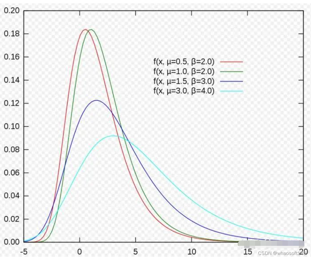
不同参数的gumbel分布的PDF函数曲线 whaosoft aiot http://143ai.com
写成代码的话,就是
import torch

# gumbel分布的CDF函数的反函数
def inverse_gumbel_cdf(u, loc, beta):
    return loc - scale * torch.log(-torch.log(u))

def gumbel_distribution_sampling(n, loc=0, scale=1):
    u = torch.rand(n)  #使用torch.rand生成均匀分布
    g = inverse_gumbel_cdf(u, loc, scale)
    return g

n = 10  # 采样个数
loc = 0 # gumbel分布的位置系数,类似于高斯分布的均值
scale = 1 # gumbel分布尺度系数,类似于高斯分布的标准差

samples = gumbel_distribution_sampling(n, loc, scale)
重参数技巧(Re-parameterization Trick)
gumbel max trick里用到了重参数的思想,所以先介绍一下重参数技巧。
最原始的自编码器(AE,Auto Encoder,自编码器就是输入一张图片,编码成一个隐向量,再把这个隐向量重建回原图的样子)长这样:
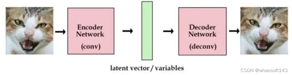
左右两边是端到端的输入输出网络,中间的绿色是提取的特征向量,这是一种直接从图片提取特征并将特征直接重建回去的方式,很符合直觉。
而VAE(Variational Auto Encoder)长这样:
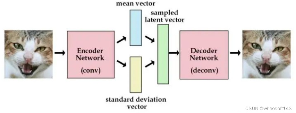 VAE的想法是不直接用编码器去提取特征向量(也就是隐向量),而是提取这张图像的分布特征,比如说均值和标准差,也就是把绿色的特征向量替换为分布的参数向量。然后需要解码图像的时候,就用编码器输出的分布参数采样得到特征向量样本,用这个样本去重建图像。
以上就是重参数技巧在图像生成领域的一个案例,可以表示为下图所示:


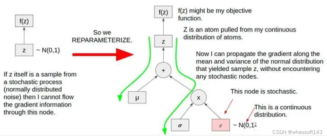 Gumbel-Max Trick
Gumbel-Max Trick也是使用了重参数技巧把采样过程分成了确定性的部分和随机性的部分,我们会计算所有类别的log分布概率(确定性的部分),类似于上面例子中的均值,然后加上一些噪音(随机性的部分),上面的例子中,噪音是标准高斯分布,而这里噪音是标准gumbel分布。在我们把采样过程的确定性部分和随机性部分结合起来之后,我们在此基础上再用一个argmax来找到具有最大概率的类别。自此可见,Gumbel-Max Trick由使用gumbel分布的Re-parameterization Trick和argmax组成而成,正如它的名字一样。
用公式表示的话就是:
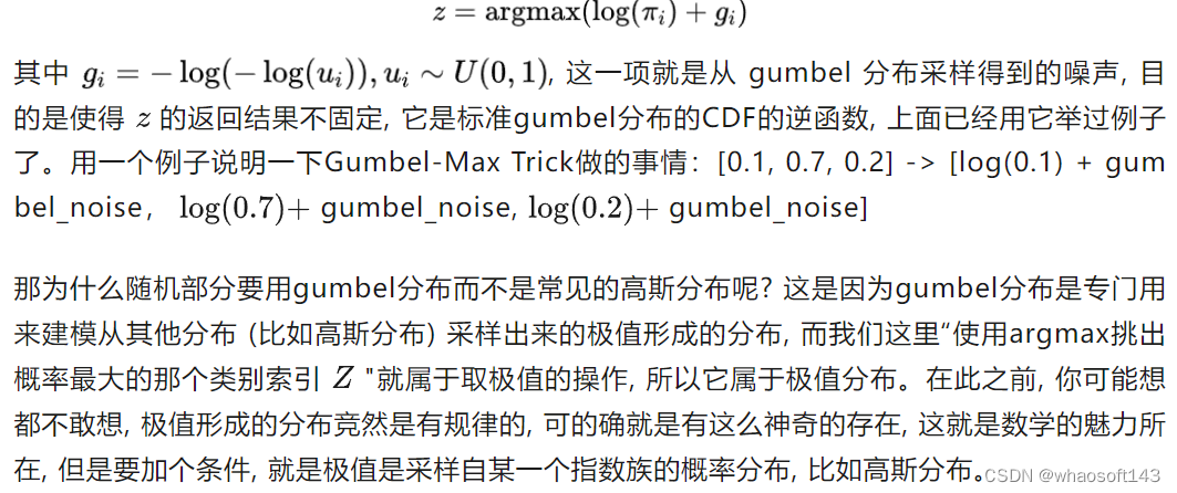 下面我们用一个例子和代码来验证一下这个极值分布的规律。假设你每天都会喝很多次水(比如100次),每次喝水的量服从正态分布N(μ,σ2)(其实也有点不合理,毕竟喝水的多少不能取为负值,不过无伤大雅能理解就好,假设均值为5),那么每天100次喝水里总会有一个最大值,这个最大值服从的分布就是Gumbel分布。
from scipy.optimize import curve_fit
import numpy as np
import matplotlib.pyplot as plt
mean_hunger = 5
samples_per_day = 100
n_days = 10000
samples = np.random.normal(loc=mean_hunger, scale=1.0, size=(n_days, samples_per_day))
daily_maxes = np.max(samples, axis=1)

# gumbel的通用PDF公式见维基百科
def gumbel_pdf(prob,loc,scale):
    z = (prob-loc)/scale
    return np.exp(-z-np.exp(-z))/scale

def plot_maxes(daily_maxes):
    probs,bins,_ = plt.hist(daily_maxes,density=True,bins=100)
    print(f"==>> probs: {probs}") # 每个bin的概率
    print(f"==>> bins: {bins}") # 即横坐标的tick值
    print(f"==>> _: {_}")
    print(f"==>> probs.shape: {probs.shape}") # (100,)
    print(f"==>> bins.shape: {bins.shape}") # (101,)
    plt.xlabel('Volume')
    plt.ylabel('Probability of Volume being daily maximum')

    # 基于直方图,下面拟合出它的曲线。

    (fitted_loc, fitted_scale), _ = curve_fit(gumbel_pdf, bins[:-1],probs)
    print(f"==>> fitted_loc: {fitted_loc}")
    print(f"==>> fitted_scale: {fitted_scale}")
    #curve_fit用于曲线拟合,doc:https://docs.scipy.org/doc/scipy/reference/generated/scipy.optimize.curve_fit.html
    #比如我们要拟合函数y=ax+b里的参数a和b,a和b确定了,这个函数就确定了,为了拟合这个函数,我们需要给curve_fit()提供待拟合函数的输入和输出样本
    #所以curve_fit()的三个入参是:1.待拟合的函数(要求该函数的第一个入参是输入,后面的入参是要拟合的函数的参数)、2.样本输入、3.样本输出
    #返回的是拟合好的参数,打包在元组里
    # 其他教程:https://blog.csdn.net/guduruyu/article/details/70313176
    plt.plot(bins, gumbel_pdf(bins, fitted_loc, fitted_scale))

plt.figure()
plot_maxes(daily_maxes)

上面的例子中极值是采样自高斯分布,且是连续分布,那如果极值是采样自一个离散的类别分布呢,下面我们再用代码来验证一下。
如下代码定义了一个7类别的多项分布,每个类别的概率如下图
n_cats = 7
cats = np.arange(n_cats)
probs = np.random.randint(low=1, high=20, size=n_cats)
probs = probs / sum(probs)
logits = np.log(probs)
def plot_probs():
    plt.bar(cats, probs)
    plt.xlabel("Category")
    plt.ylabel("Probability")
plt.figure()
plot_probs()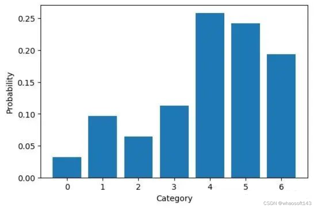

def sample_gumbel(logits):
noise = np.random.gumbel(size=len(logits))
sample = np.argmax(logits+noise)
return sample
gumbel_samples = [sample_gumbel(logits) for _ in range(n_samples)]
def sample_uniform(logits):
noise = np.random.uniform(size=len(logits))
sample = np.argmax(logits+noise)
return sample
uniform_samples = [sample_uniform(logits) for _ in range(n_samples)]
def sample_normal(logits):
noise = np.random.normal(size=len(logits))
sample = np.argmax(logits+noise)
return sample
normal_samples = [sample_normal(logits) for _ in range(n_samples)]
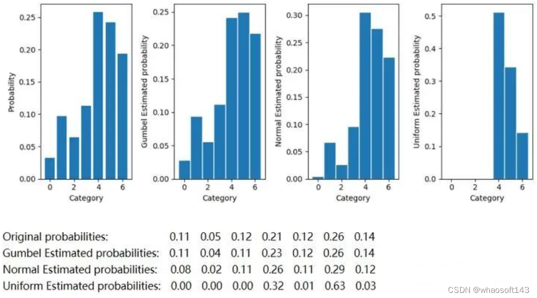
plt.figure(figsize=(10,4))
plt.subplot(1,4,1)
plot_probs()
plt.subplot(1,4,2)
gumbel_estd_probs = plot_estimated_probs(gumbel_samples,'Gumbel ')
plt.subplot(1,4,3)
normal_estd_probs = plot_estimated_probs(normal_samples,'Normal ')
plt.subplot(1,4,4)
uniform_estd_probs = plot_estimated_probs(uniform_samples,'Uniform ')
plt.tight_layout()
print('Original probabilities:\t\t',end='')
print_probs(probs)
print('Gumbel Estimated probabilities:\t',end='')
print_probs(gumbel_estd_probs)
print('Normal Estimated probabilities:\t',end='')
print_probs(normal_estd_probs)
print('Uniform Estimated probabilities:',end='')
print_probs(uniform_estd_probs)
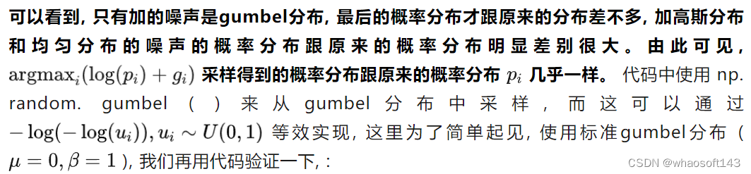
n_samples = 100000
numpy_gumbel = np.random.gumbel(loc=0, scale=1.0, size=n_samples)
manual_gumbel = -np.log(-np.log(np.random.uniform(size=n_samples)))
plt.figure()
plt.subplot(1, 2, 1)
plt.hist(numpy_gumbel, bins=50)
plt.ylabel("Probability")
plt.xlabel("numpy Gumbel")
plt.subplot(1, 2, 2)
plt.hist(manual_gumbel, bins=50)
plt.xlabel("Gumbel from uniform noise")
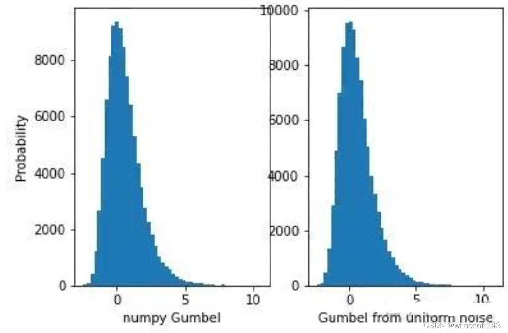
可以看到,两个分布几乎一模一样。

Gumbel Softmax
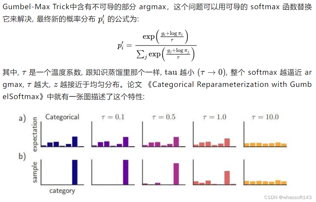
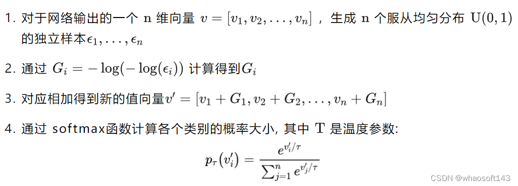
最后总结一下Gumbel-Softmax Trick的步骤:
其实我觉得只是把argmax替换成softmax还不够,应该是替换成soft argmax,这一点有待以后如果工作中遇到了再验证。也欢迎有实践经验的朋友告知。
pytorch相关函数说明
pytorch 提供的torch.nn.functional.gumbel_softmax api:https://pytorch.org/docs/stable/generated/torch.nn.functional.gumbel_softmax.html#torch.nn.functional.gumbel_softmax
视频讲解:《Gumbel Softmax补充说明》
实现的源代码:https://pytorch.org/docs/stable/_modules/torch/nn/functional.html#gumbel_softmax
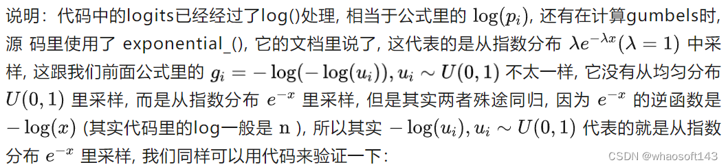
我这里对实现的源代码做一些说明:
gumbels = (
        -torch.empty_like(logits, memory_format=torch.legacy_contiguous_format).exponential_().log()
    )  # ~Gumbel(0,1)
    gumbels = (logits + gumbels) / tau  # ~Gumbel(logits,tau)
    y_soft = gumbels.softmax(dim)

    if hard:
        # Straight through.
        index = y_soft.max(dim, keepdim=True)[1]
        y_hard = torch.zeros_like(logits, memory_format=torch.legacy_contiguous_format).scatter_(dim, index, 1.0)
        ret = y_hard - y_soft.detach() + y_soft
    else:
        # Reparametrization trick.
        ret = y_soft
    return ret
import numpy as np
import matplotlib.pyplot as plt
n_samples = 100000
numpy_exponential = np.random.exponential(size=n_samples)
manual_exponential = -np.log(np.random.uniform(size=n_samples))
plt.figure()
plt.subplot(1, 2, 1)
plt.hist(numpy_exponential, bins=50)
plt.ylabel("Probability")
plt.xlabel("numpy exponential")
plt.subplot(1, 2, 2)
plt.hist(manual_exponential, bins=50)
plt.xlabel("Exponential from uniform noise")
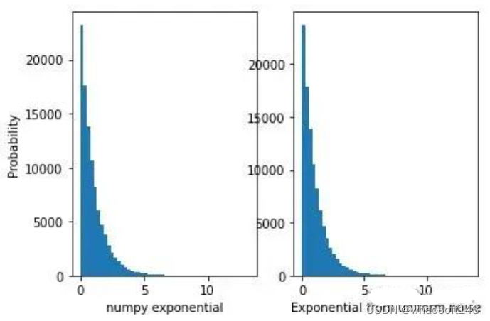 可以看到两个分布十分近似,所以pytorch源代码里使用指数分布采样是没问题的。
本文部分内容参考或摘抄自:
《gumber分布的维基百科》
《Gumbel-Softmax 完全解析》
《Gumbel-Softmax Trick和Gumbel分布 》
《The Gumbel-Softmax Distribution》
《Gumbel softmax trick (快速理解附代码)》
《漫谈重参数:从正态分布到Gumbel Softmax》