鸢尾花数据集
目录
一、鸢尾花数据集是什么?
鸢尾花数据集是一个经典数据集,在统计学习和机器学习领域都经常被用作例子。数据集内包含 3 类共 150 个样本,每类各 50 个样本,每条样本都有 4 个特征:花萼长度、花萼宽度、花瓣长度、花瓣宽度,可以通过这 4 个特征预测鸢尾花属于(iris-setosa, iris-versicolour, iris-virginica)中的哪个品种。

二、使用python获取鸢尾花数据集
1.数据集的获取及展示
from sklearn.datasets import load_iris #需要通过该语句在库中获取 或者网上寻找该文件,我已上传到资源区(iris)
from sklearn.datasets import load_iris

#1.数据集的获取
#1.1小数据集获取
iris=load_iris()
#print(iris)

# 2.数据集属性描述
print("数据集中的特征值是:\n",iris.data)
print("数据集中的目标值是:\n",iris["target"])
print("数据集中的特征值的名字是:\n",iris.feature_names)
print("数据集中的目标值的名字是:\n",iris.target_names)
print("数据集的描述:\n",iris.DESCR)
以下为部分结果(参考):
数据集中的特征值是:
[[5.1 3.5 1.4 0.2]
[4.9 3. 1.4 0.2]
[4.7 3.2 1.3 0.2]
[4.6 3.1 1.5 0.2]
[5. 3.6 1.4 0.2]
[5.4 3.9 1.7 0.4]
[4.6 3.4 1.4 0.3]
[5. 3.4 1.5 0.2]
......
......
[6.5 3. 5.2 2. ]
[6.2 3.4 5.4 2.3]
[5.9 3. 5.1 1.8]]
数据集中的目标值是:
[0 0 0 0 0 0 0 0 0 0 0 0 0 0 0 0 0 0 0 0 0 0 0 0 0 0 0 0 0 0 0 0 0 0 0 0 0
0 0 0 0 0 0 0 0 0 0 0 0 0 1 1 1 1 1 1 1 1 1 1 1 1 1 1 1 1 1 1 1 1 1 1 1 1
1 1 1 1 1 1 1 1 1 1 1 1 1 1 1 1 1 1 1 1 1 1 1 1 1 1 2 2 2 2 2 2 2 2 2 2 2
2 2 2 2 2 2 2 2 2 2 2 2 2 2 2 2 2 2 2 2 2 2 2 2 2 2 2 2 2 2 2 2 2 2 2 2 2
2 2]
数据集中的特征值的名字是:
['sepal length (cm)', 'sepal width (cm)', 'petal length (cm)', 'petal width (cm)']
数据集中的目标值的名字是:
['setosa' 'versicolor' 'virginica']
数据集的描述:
.. _iris_dataset:
Iris plants dataset
--------------------
**Data Set Characteristics:**
:Number of Instances: 150 (50 in each of three classes)
:Number of Attributes: 4 numeric, predictive attributes and the class
:Attribute Information:
- sepal length in cm
- sepal width in cm
- petal length in cm
- petal width in cm
- class:
- Iris-Setosa
- Iris-Versicolour
- Iris-Virginica
:Summary Statistics:
============== ==== ==== ======= ===== ====================
Min Max Mean SD Class Correlation
============== ==== ==== ======= ===== ====================
sepal length: 4.3 7.9 5.84 0.83 0.7826
sepal width: 2.0 4.4 3.05 0.43 -0.4194
petal length: 1.0 6.9 3.76 1.76 0.9490 (high!)
petal width: 0.1 2.5 1.20 0.76 0.9565 (high!)
============== ==== ==== ======= ===== ====================
:Missing Attribute Values: None
:Class Distribution: 33.3% for each of 3 classes.
:Creator: R.A. Fisher
:Donor: Michael Marshall (MARSHALL%[email protected])
:Date: July, 1988
2.数据可视化及获得一元线性回归
import seaborn as sns
import matplotlib.pyplot as plt
import pandas as pd
from sklearn.datasets import load_iris
#1.数据集的获取
#1.1小数据集获取
iris=load_iris()
#3.数据可视化
#3.1 数据类型的转换,把数据用DataFrame储存
iris_data=pd.DataFrame(data=iris.data,columns=['Sepal_Length','Sepal_Width','Petal_Length','Petal_Width'])
iris_data["target"]=iris.target
#print(iris_data)
def iris_plot(data,col1,col2):
    sns.lmplot(x=col1,y=col2,data=data,hue="target")
    plt.rcParams['font.sans-serif']=['SimHei'] #用来正常显示中文标签
    plt.title('鸢尾花数据展示')
    plt.xlabel(col1)
    plt.ylabel(col2)
    plt.show()

iris_plot(iris_data,"Sepal_Length","Petal_Width")
iris_plot(iris_data,'Sepal_Length','Sepal_Width')

可发现按照不同的x,y所得结果得区分度不同
3.数据集的划分
import pandas as pd
from sklearn.datasets import load_iris
from sklearn.model_selection import train_test_split
iris_data=pd.DataFrame(data=iris.data,columns=['Sepal_Length','Sepal_Width','Petal_Length','Petal_Width'])
iris_data["target"]=iris.target
#数据集的划分
x_train,x_test,y_train,y_test=train_test_split(iris_data,iris.target,test_size=0.2,random_state=2)
print("训练集的特征值:\n",x_train)
print("测试集的特征值:\n",x_test)
print("训练集的目标值:\n",y_train)
print("测试集的目标值:\n",y_test)

print("训练集的目标值形状:\n",y_train.shape)
print("测试集的目标值形状:\n",y_test.shape)
运行结果(部分):
训练集的特征值:
Sepal_Length Sepal_Width Petal_Length Petal_Width target
126 6.2 2.8 4.8 1.8 2
23 5.1 3.3 1.7 0.5 0
64 5.6 2.9 3.6 1.3 1
117 7.7 3.8 6.7 2.2 2
84 5.4 3.0 4.5 1.5 1
.. ... ... ... ... ...
75 6.6 3.0 4.4 1.4 1
43 5.0 3.5 1.6 0.6 0
22 4.6 3.6 1.0 0.2 0
72 6.3 2.5 4.9 1.5 1
15 5.7 4.4 1.5 0.4 0
[120 rows x 5 columns]
测试集的特征值:
Sepal_Length Sepal_Width Petal_Length Petal_Width target
6 4.6 3.4 1.4 0.3 0
3 4.6 3.1 1.5 0.2 0
113 5.7 2.5 5.0 2.0 2
12 4.8 3.0 1.4 0.1 0
24 4.8 3.4 1.9 0.2 0
.. ... ... ... ... ...
29 4.7 3.2 1.6 0.2 0
2 4.7 3.2 1.3 0.2 0
127 6.1 3.0 4.9 1.8 2
44 5.1 3.8 1.9 0.4 0
125 7.2 3.2 6.0 1.8 2
训练集的目标值:
[2 0 1 2 1 0 2 1 1 2 1 1 2 1 0 2 0 1 0 0 0 2 2 2 0 2 2 2 2 0 0 2 1 1 2 2 1
0 1 0 2 1 1 0 1 1 1 2 0 1 0 1 2 0 1 0 0 0 2 2 0 0 2 2 1 2 1 1 2 0 2 2 2 0
2 0 0 1 2 1 2 1 1 2 1 1 1 2 1 2 1 0 1 1 1 1 2 1 0 0 2 1 2 0 2 0 2 2 0 1 0
2 1 0 2 1 0 0 1 0]
测试集的目标值:
[0 0 2 0 0 2 0 2 2 0 0 0 0 0 1 1 0 1 2 1 1 1 2 1 1 0 0 2 0 2]
训练集的目标值形状:
(120,)
测试集的目标值形状:
(30,)
三、鸢尾花数据集使用三种梯度下降BGD、SGD与MBGD
BGD:
# -*- coding: utf-8 -*-
"""
Created on Tue Apr 11 11:35:33 2023
@author: Lenovo
"""
import numpy as np
import pandas as pd
import matplotlib.pyplot as plt
from sklearn.datasets import load_iris
# 加载数据集
iris = load_iris()
X = iris.data[:, 2] # 取花瓣长度特征
y = iris.data[:, 3]
# 数据标准化
X = (X - np.mean(X)) / np.std(X)
# 构建模型
theta = np.zeros(2) # 参数初始化
alpha = 0.01 # 学习率
iters = 1000 # 迭代次数
m = len(X) # 样本数量
# 批量梯度下降算法
def bgd(X, y, theta, alpha, iters):
J_history = [] # 记录代价函数的值
for i in range(iters):
h = np.dot(X, theta) # 预测值
error = h - y # 误差
cost = 1 / (2 * m) * np.dot(error.T, error) # 计算代价函数
J_history.append(cost)
theta = theta - (alpha / m) * np.dot(X.T, error) # 更新参数
return theta, J_history
# 训练模型
X = np.c_[np.ones(m), X] # 增加一列全为1的特征
theta, J_history = bgd(X, y, theta, alpha, iters)
print("theta: ", theta)
# 可视化
plt.scatter(X[:, 1], y)
plt.plot(X[:, 1], np.dot(X, theta), color='r')
plt.xlabel('Petal length')
plt.ylabel('Target')
plt.show()
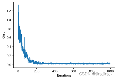
# 绘制代价函数随迭代次数变化的曲线
plt.plot(np.arange(iters), J_history)
plt.xlabel('Iterations')
plt.ylabel('Cost')
plt.show()结果:


SGD:
# -*- coding: utf-8 -*-
"""
Created on Tue Apr 11 11:41:34 2023

@author: Lenovo
"""

import numpy as np
import pandas as pd
import matplotlib.pyplot as plt
from sklearn.datasets import load_iris

# 加载数据集
iris = load_iris()
X = iris.data[:, 2]  # 取花瓣长度特征
y = iris.data[:, 1]
# y = iris.target

# 数据标准化
X = (X - np.mean(X)) / np.std(X)

# 构建模型
theta = np.zeros(2)  # 参数初始化
alpha = 0.01  # 学习率
iters = 100  # 迭代次数
m = len(X)  # 样本数量

# 随机梯度下降算法
def sgd(X, y, theta, alpha, iters):
    J_history = []  # 记录代价函数的值
    for i in range(iters):
        for j in range(m):
            h = np.dot(X[j], theta)  # 预测值
            error = h - y[j]  # 误差
            cost = 1 / 2 * error ** 2  # 计算代价函数
            J_history.append(cost)
            theta = theta - alpha * error * X[j]  # 更新参数
    return theta, J_history

# 训练模型
X = np.c_[np.ones(m), X]  # 增加一列全为1的特征
theta, J_history = sgd(X, y, theta, alpha, iters)
print("theta: ", theta)

# 可视化
plt.scatter(X[:, 1], y)
plt.plot(X[:, 1], np.dot(X, theta), color='r')
plt.xlabel('Petal length')
plt.ylabel('Target')
plt.show()

# 绘制代价函数随迭代次数变化的曲线
plt.plot(np.arange(m * iters), J_history)
plt.xlabel('Iterations')
plt.ylabel('Cost')
plt.show()
结果:


MBGD:
# -*- coding: utf-8 -*-
"""
Created on Tue Apr 11 11:41:24 2023

@author: Lenovo
"""

import numpy as np
import pandas as pd
import matplotlib.pyplot as plt
from sklearn.datasets import load_iris

# 加载数据集
iris = load_iris()
X = iris.data[:, 2]  # 取花瓣长度特征
y = iris.data[:, 3]

# 数据标准化
X = (X - np.mean(X)) / np.std(X)

# 构建模型
theta = np.zeros(2)  # 参数初始化
alpha = 0.01  # 学习率
iters = 1000  # 迭代次数
batch_size = 16  # 小批量大小
m = len(X)  # 样本数量

# 小批量梯度下降算法
def mini_batch_gd(X, y, theta, alpha, iters, batch_size):
    J_history = []  # 记录代价函数的值
    for i in range(iters):
        # 从样本中随机选择一个小批量
        idx = np.random.choice(m, batch_size, replace=False)
        X_batch = X[idx]
        y_batch = y[idx]
        h = np.dot(X_batch, theta)  # 预测值
        error = h - y_batch  # 误差
        cost = 1 / (2 * batch_size) * np.dot(error.T, error)  # 计算代价函数
        J_history.append(cost)
        theta = theta - (alpha / batch_size) * np.dot(X_batch.T, error)  # 更新参数
    return theta, J_history

# 训练模型
X = np.c_[np.ones(m), X]  # 增加一列全为1的特征
theta, J_history = mini_batch_gd(X, y, theta, alpha, iters, batch_size)
print("theta: ", theta)

# 可视化
plt.scatter(X[:, 1], y)
plt.plot(X[:, 1], np.dot(X, theta), color='r')
plt.xlabel('Petal length')
plt.ylabel('Target')
plt.show()

# 绘制代价函数随迭代次数变化的曲线
plt.plot(np.arange(iters), J_history)
plt.xlabel('Iterations')
plt.ylabel('Cost')
plt.show()
结果:

得出结论:
批量梯度下降法(Batch Gradient Descent)
批量梯度下降法(BGD)每次都使用训练集中的所有样本更新参数。它得到的是一 个全局最优解,但是每迭代一步,都要用到训练集所有的数据,如果m很大,那么迭代速度就会变得很慢。
优点:可以得出全局最优解。
缺点:样本数据集大时,训练速度慢。
随机梯度下降法(Stochastic Gradient Descent)
随机梯度下降法(SGD)每次更新都从样本随机选择1组数据,因此随机梯度下降比 批量梯度下降在计算量上会大大减少。
SGD有一个缺点是,其噪音较BGD 要多,使得SGD并不是每次迭代都向着整体最优化方向。而且SGD因为每 次都是使用一个样本进行迭代,因此最终求得的最优解往往不是全局最优 解,而只是局部最优解。但是大的整体的方向是向全局最优解的,最终的结果往往是在全局最优解附近。
优点:训练速度较快。
缺点:过程杂乱,准确度下降。
小批量梯度下降法(Mini-batch Gradient Descent)
小批量梯度下降法(MBGD)对包含n个样本的数据集进行计算。综合了上述两种方法,既保证了训练速度快,又保证了准确度。
四、什么是数据集(测试集,训练集和验证集)
数据集常被分成2~3个,即:训练集(train set),验证集(validation set),测试集(test set)。

如果给定的样本数据充足,我们通常使用均匀随机抽样的方式将数据集划分成3个部分——训练集、验证集和测试集,这三个集合不能有交集,常见的比例是8:1:1。需要注意的是,通常都会给定训练集和测试集,而不会给验证集。这时候验证集该从哪里得到呢?一般的做法是,从训练集中均匀随机抽样一部分样本作为验证集。
训练集
训练集用来训练模型,即确定模型的权重和偏置这些参数,通常我们称这些参数为学习参数。
验证集
而验证集用于模型的选择,更具体地来说,验证集并不参与学习参数的确定,也就是验证集并没有参与梯度下降的过程。验证集只是为了选择超参数,比如网络层数、网络节点数、迭代次数、学习率这些都叫超参数。比如在k-NN算法中,k值就是一个超参数。所以可以使用验证集来求出误差率最小的k。
测试集
测试集只使用一次,即在训练完成后评价最终的模型时使用。它既不参与学习参数过程,也不参数超参数选择过程,而仅仅使用于模型的评价。
值得注意的是,千万不能在训练过程中使用测试集,而后再用相同的测试集去测试模型。这样做其实是一个cheat,使得模型测试时准确率很高。
参考文献
[EB/OL].https://blog.csdn.net/HaoZiHuang/article/details/104819026,2020-3-12
[EB/OL].11 鸢尾花数据可视化_哔哩哔哩_bilibili,2020-1-22