基于libtorch的yolov5目标检测网络实现(2)——网络结构实现

“yolov5是yolo系列目标检测框架的v5版本，本系列文章我们将一步步来解析该框架的原理，并使用libtorch来一步步将其实现——从数据集准备，到网络结构实现，接着到损失函数实现，再到训练代码实现，最后到模型验证。”

上篇文章中我们已经讲了COCO数据集的json标签文件的解析：

基于libtorch的yolov5目标检测网络实现——COCO数据集json标签文件解析
 

本文我们主要讲yolov5网络的结构与实现。

01 yolov5网络目标检测的基本思想

yolov5网络输入640*640的三通道图像，也即3*640*640的矩阵数据，如果原图像尺寸不是640*640，则通过填充或缩放将其尺寸变成640*640尺寸之后再输入网络。

通常把640*640的图像划分成N*N（通常为80*80，或40*40，或20*20）的网格区域。网络的输出端则输出所有网格区域的预测信息，每个网格的预测信息包括目标的分类概率、置信度，以及包围检测目标的方框的中心坐标、长、宽。其中分类概率表征网格区域所预测目标的分类信息，置信度表征网格区域中存在检测目标的概率（也即置信度越高表示该网格区域越有可能存在检测目标），方框的中心坐标、长、宽信息则表示网格所预测目标的具体大小和位置。

因此，在解析网络输出时，我们根据每个网格的置信度是否超过设定阈值来判断该网格区域是否有检测目标（并非每个网格区域都存在检测目标），根据分类概率来判断该网格所预测目标的分类，根据方框信息来确定目标的位置和大小。

由于检测目标有大有小、尺度不一，通常使用不同的网格尺寸同时对640*640图像进行区域划分，小尺寸网格负责检测小目标，大尺寸网格负责检测大目标，比如yolov5网络将640*640图像分别划分为80*80-->40*40-->20*20的网格，对应的网格尺寸分别为8*8-->16*16-->32*32，不同尺寸网格负责预测目标的尺寸分别为小-->中-->大。

此外，每一个网格会预测3个不同尺寸和位置的检测目标（这3个目标的尺寸属同一级别，位置都在同一网格内，但具体尺寸和坐标位置则不相同），因此：

• 80*80网格输出3*80*80个小尺寸检测目标的信息

• 40*40网格输出3*40*40个中尺寸检测目标的信息

• 20*20网格输出3*20*20个大尺寸检测目标的信息

02 yolov5整体网络结构

如下图所示，yolov5的网络结构主要由输入端、Backbone、Neck、Head这4大部分组成（其中nc为分类总数，比如COCO数据集总共有80个分类，那么nc=80）。

其中各部分的作用为：

• 输入端：对输入图像进行填充或缩放，使其尺寸变成3*640*640，并对图像数据进行归一化，转换为0~1之间的浮点数；

• Backbone：提取图像特征；

• Neck：Neck在Backbone和Head之间，其作用为对Backbone输出的图像特征信息进行进一步提取、融合；

• Head：对Neck输出的特征信息进行分类、定位，从而输出检测目标的分类概率、置信度、方框等信息。

以上是从大组件的角度来对网络结构进行解析，如果更加细分，我们会发现整个网络又主要由Focus、CBL、CSP1_n、SPP、CSP2_n、Upsample和Conv这几个小组件搭建而成(图中的cat为张量的拼接操作，前文已经讲过，此处不再重复)。因此主要把这几个小组件实现之后，那么整个网络就容易实现了。在以下章节中我们将分别讲解这几个组件的结构与实现。

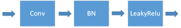
03 CBL结构与实现

CBL组件由1个卷积层（Conv层）、1个Batch normalize层（BN层），和1个LeakyRelu激活函数层构成，如下图所示：

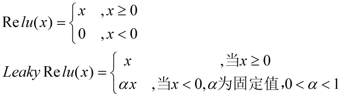
这里的LeakyRelu激活函数是后人在Relu函数的基础上新提出的，我们对比一下它们的计算公式：

两者的函数曲线分别为：

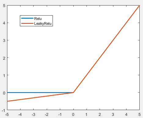
可以看到两种激活函数的主要区别在于输入小于0的情况，此情况下Relu直接输出0，而LeakyRelu则输出固定系数与输入信号的乘积，因此LeakyRelu解决了Relu在输入小于0时梯度死亡的问题。

CBL代码实现：

#define NONE -1


//自动计算padding参数，当输入的padding参数为-1时，则取卷积核尺寸的一半作为padding参数
int autopad(int k, int p)
{
  if (p == NONE)
    return k / 2;
  else
    return p;
}


struct CBL :torch::nn::Module
{


  bool _act;   //_act参数控制输出是否经过LeakyRelu激活


  CBL(int c1, int c2, int k = 1, int s = 1, int p = NONE, int g = 1, bool act = true, float e = 1.0)
  {


    int _c1 = (int)(c1*e + 0.5);
    int _c2 = (int)(c2*e + 0.5);
    _act = act;


    conv1 = register_module("conv1", torch::nn::Conv2d(torch::nn::Conv2dOptions(_c1, _c2, k).stride(s).padding(autopad(k, p)).groups(g).bias(false)));


    c1b = register_module("c1b", torch::nn::BatchNorm2d(torch::nn::BatchNorm2dOptions(_c2).eps(1e-5).momentum(0.1).affine(true).track_running_stats(true)));
  }


  torch::Tensor forward(torch::Tensor input)
  {
    namespace F = torch::nn::functional;


    auto x = conv1->forward(input);


    x = c1b->forward(x);


    if (_act)
    {
      x = torch::nn::LeakyReLU(torch::nn::LeakyReLUOptions().negative_slope(1e-2).inplace(true))->forward(x);
    }
      


    return x;
  }


  torch::nn::Conv2d conv1{ nullptr };
  torch::nn::BatchNorm2d c1b{ nullptr };


};

04 Focus结构与实现

Focus主要是对输入的[3, 640, 640]数据以2的间隔在第2维度、第3维度上面进行slice切片，然后将切片之后的数据在第1维度上面拼接，如下图所示：

所以Focus相当于对每个通道图像进行2倍下采样，然后再对下采样图像进行拼接的操作，最后将拼接之后的数据输入CBL进行处理。

代码实现：

struct Focus :torch::nn::Module
{


  Focus(int c1, int c2, int k = 3, int s = 1, int p = 1, int g = 1, bool act = true, float e = 1.0)
  {
    int _c2 = (int)(c2*e + 0.5);
    cbl_s = register_module("cbl_s", torch::nn::Sequential(CBL(c1 * 4, _c2, k, s, p, g, act)));
  }




  torch::Tensor forward(torch::Tensor input)
{


    auto x = torch::cat({ input.index({ "...", Slice({0, None, 2}), Slice({0, None, 2}) }),
                          input.index({ "...", Slice({1, None, 2}), Slice({0, None, 2}) }),
                          input.index({ "...", Slice({0, None, 2}), Slice({1, None, 2}) }),
                          input.index({ "...", Slice({1, None, 2}), Slice({1, None, 2}) }) }, 1);


    x = cbl_s->forward(x);


    return x;
  }




  torch::nn::Sequential cbl_s{ nullptr };
};

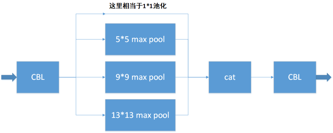
05 SPP结构与实现

SPP是空间金字塔池化的缩写，SPP模块的精髓在于使用不同尺寸的池化窗口分别对数据进行池化操作，然后再对不同池化窗口的池化结果进行拼接。主要有以下两个作用：

• 解决对输入图像进行裁剪、缩放导致的图像失真问题；

• 通过不同尺度的池化、融合，有利于在检测目标大小差异较大情况下的目标检测。

SPP的主要构成如下图所示：

代码实现：

struct SPP :torch::nn::Module
{
  int _k1, _k2, _k3;


  SPP(int c1, int c2, int k1 = 5, int k2 = 9, int k3 = 13, float e = 1.0)
  {
    int _c1 = (int)(c1*e + 0.5);
    int _c2 = (int)(c2*e + 0.5);
    int _c = _c1 / 2;
    _k1 = k1;
    _k2 = k2;
    _k3 = k3;


    cbl_before = register_module("cbl_before", torch::nn::Sequential(CBL(_c1, _c, 1, 1)));
    cbl_after = register_module("cbl_after", torch::nn::Sequential(CBL(_c * 4, _c2, 1, 1)));
  }




  torch::Tensor forward(torch::Tensor input)
{


    namespace F = torch::nn::functional;
    //CBL输出，相当于1*1池化
    auto x0 = cbl_before->forward(input);   //CBL
    //5*5池化
    auto x1 = F::max_pool2d(x0, F::MaxPool2dFuncOptions(_k1).stride(1).padding(_k1 / 2));
    //9*9池化
    auto x2 = F::max_pool2d(x0, F::MaxPool2dFuncOptions(_k2).stride(1).padding(_k2 / 2));
    //13*13池化
    auto x3 = F::max_pool2d(x0, F::MaxPool2dFuncOptions(_k3).stride(1).padding(_k3 / 2));
    //将1*1、5*5、9*9、13*13的池化结果进行拼接
    auto x_cat = torch::cat({ x0, x1, x2, x3 }, 1);
    //将拼接结果再输入CBL
    x_cat = cbl_after->forward(x_cat);


    return x_cat;
  }


  torch::nn::Sequential cbl_before{ nullptr };
  torch::nn::Sequential cbl_after{ nullptr };
};

06 CSP1_n和CSP2_n结构与实现

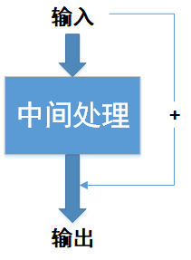
讲CSP1_n和CSP2_n的结构之前，让我们先来回顾一下残差模块，之前我们在Resnet34网络中已经讲过残差模块：

基于libtorch的Resnet34残差网络实现——Cifar-10分类

残差模块的主要特点是把输入信号加到输出信号中，如下图所示：

我们把CSP1_n中的残差模块称为ResUnit_n模块，ResUnit_n模块中包含了2的倍数个CBL模块，如下图所示：

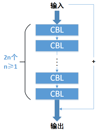
而CSP1_n中又包含了n个ResUnit_n模块，比如CSP1_1有1个ResUnit_n，CSP1_3有3个ResUnit_n：

CSP2_n与CSP1_n模块的结构大同小异，唯一的区别在于ResUnit_n残差模块：CSP1_n中的ResUnit_n模块把输入信号叠加到输出，而CSP2_n中的ResUnit_n模块则不把输入信号迭代到输出。如下图所示：

因此在实现代码的时候，我们可以给ResUnit_n模块增加一个参数，用于控制是否把输入信号叠加到输出上：该参数为true则叠加，为false则不叠加。这样一来，CSP2_n与CSP1_n模块就可以使用同一段代码来实现了，区别在于传入的参数是true还是false：

//残差模块代码
//参数res_flag控制是否把输入信号叠加到输出上
struct ResUnit_n :torch::nn::Module
{


  bool _shortcut;
  bool _res_flag;


  ResUnit_n(int c1, int c2, int n, bool res_flag = true)
  {
    _shortcut = (c1 == c2) ? true : false;
    _res_flag = res_flag;


    res_n = register_module("res_n", torch::nn::Sequential());


    for (int i = 0; i < n; i++)
    {
      res_n->push_back(CBL(c1, c1, 1, 1, 0));
      res_n->push_back(CBL(c1, c2, 3, 1, 1));
    }


  }


  torch::Tensor forward(torch::Tensor input)
{
    Tensor x;


    if (_shortcut && _res_flag)
      x = input + res_n->forward(input);
    else
      x = res_n->forward(input);


    return x;
  }


  torch::nn::Sequential res_n{ nullptr };
};


//CSP1_n与CSP2_n模块代码，res_flag为true是CSP1_n，res_flag为false是CSP2_n
struct CSP1_n :torch::nn::Module
{


  CSP1_n(int c1, int c2, int k = 1, int s = 1, int p = NONE, int g = 1, bool act = true, bool res_flag = true, int n = 1, float e0 = 1.0, float e1 = 1.0)
  {
    int _n = (int)(n*e0 + 0.5);
    int _c1 = (int)(c1*e1 + 0.5);
    int _c2 = (int)(c2*e1 + 0.5);
    int _c = _c2 / 2;


    up = register_module("up", torch::nn::Sequential(
      CBL(_c1, _c, k, s, autopad(k, p), g, act),
      ResUnit_n(_c, _c, _n, res_flag)
      //torch::nn::Conv2d(torch::nn::Conv2dOptions(_c, _c, 1).stride(1).padding(0).bias(false))
    ));


    bottom = register_module("bottom", torch::nn::Conv2d(torch::nn::Conv2dOptions(_c1, _c, 1).stride(1).padding(0)));


    tie = register_module("tie", torch::nn::Sequential(
      torch::nn::BatchNorm2d(torch::nn::BatchNorm2dOptions(_c * 2).eps(1e-5).momentum(0.1).affine(true).track_running_stats(true)),
      torch::nn::LeakyReLU(torch::nn::LeakyReLUOptions().negative_slope(1e-2).inplace(true)),
      torch::nn::Conv2d(torch::nn::Conv2dOptions(_c * 2, _c2, 1).stride(1).padding(0).bias(false))
    ));
  }


  torch::Tensor forward(torch::Tensor input)
{
    auto x1 = up->forward(input);
    auto x2 = bottom->forward(input);
    auto total = torch::cat({ x1, x2 }, 1);


    auto x = tie->forward(total);


    return x;
  }


  torch::nn::Sequential up{ nullptr };
  torch::nn::Conv2d bottom{ nullptr };
  torch::nn::Sequential tie{ nullptr };
};

07 Upsample结构与实现

Upsample模块就是一个向上采样的操作，相当于采用插值的方式把图像放大了，比如本来图像是32*32大小，经过向上采样之后则变成64*64大小。

代码实现：

struct Up_Sample :torch::nn::Module
{
  Up_Sample()
  {
    //torch::kNearest表示使用最邻近插值的方式向上采样
    up_sample = register_module("up_sample", torch::nn::Upsample(torch::nn::UpsampleOptions().scale_factor(std::vector<double>({ 2, 2 })).mode(torch::kNearest)));
  }


  torch::Tensor forward(torch::Tensor input)
{
    auto x = up_sample->forward(input);


    return x;
  }


  torch::nn::Upsample up_sample{ nullptr };


};

08 整体网络结构与实现

以上讲整体结构时，我们说到yolov5网络大致可以分为输入端、Backbone、Neck、Head这4大部分。我们实现代码的时候，就不这么看了，我们根据输出信号的分支，把输出信号标记为out1~out7，然后以out1~out7信号的计算为导向来实现代码，如下图所示：

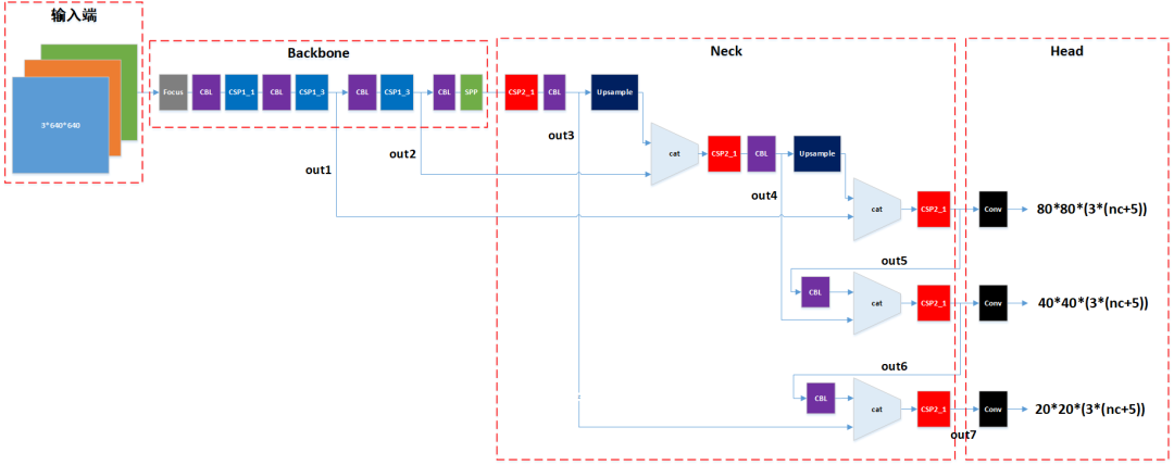
首先我们把out1~out7信号的计算分解步骤：

• Input-->Focus-->CBL-->CSP1_1-->CBL-->CSP1_3-->out1

• out1-->CBL-->CSP1_3-->out2

• out2-->CBL-->SPP-->CSP2_1-->CBL-->out3

• out3-->upsample-->upsample(out3)-->cat(upsample(out3, out2))-->CSP2_1-->CBL-->out4

• out4-->upsample-->upsample(out4)-->cat(upsample(out4, out1))-->CSP2_1-->out5

• out5-->CBL-->out5'-->cat(out5', out4)-->CSP2_1-->out6

• out6-->CBL-->out6'-->cat(out6', out3)-->CSP2_1-->out7

最后，再把out5、out6、out7分别经过一个卷积层处理，分别得到80*80、40*40、20*20网格的预测输出：

• out5-->Conv-->batch_size*80*80*255输出

• out6-->Conv-->batch_size*40*40*255输出

• out7-->Conv-->batch_size*20*20*255输出

注意到输出数据的最后一个维度都是255，这个255是怎么来的呢？COCO数据集总共有80个分类，因此输出包含80个分类概率，加上预测目标的方框信息（中心x坐标、中心y坐标、长、宽），再加上一个置信度，所以每个预测目标总共有4+1+80=85个数据，再加上每个网格预测3个目标，所以85再乘以3得到255个数据。

为了方便后续的数据分析，我们把输出的预测数据转换成以下维度：

代码实现：

struct yolov5 :torch::nn::Module
{
  int _nc;  
  //nc为分类总数，gd为控制网络深度参数，gw为控制网络宽度参数
  yolov5(int nc = 80, float gd = 0.33, float gw = 0.5)
  {
    _nc = nc;
    
    out1 = register_module("out1", torch::nn::Sequential(
      Focus(3, 64, 3, 1, 1, 1, true, gw),
      CBL(64, 128, 3, 2, 1, 1, true, gw),
      CSP1_n(128, 128, 1, 1, NONE, 1, true, true, 3, gd, gw),
      CBL(128, 256, 3, 2, 1, 1, true, gw),
      CSP1_n(256, 256, 1, 1, NONE, 1, true, true, 9, gd, gw)
    ));


    out2 = register_module("out2", torch::nn::Sequential(
      CBL(256, 512, 3, 2, 1, 1, true, gw),
      CSP1_n(512, 512, 1, 1, NONE, 1, true, true, 9, gd, gw)
    ));


    out3 = register_module("out3", torch::nn::Sequential(
      CBL(512, 1024, 3, 2, 1, 1, true, gw),
      SPP(1024, 1024, 5, 9, 13, gw),
      CSP1_n(1024, 1024, 1, 1, NONE, 1, true, false, 3, gd, gw),
      CBL(1024, 512, 1, 1, 0, 1, true, gw)
    ));
    
    upsample1 = register_module("upsample1", torch::nn::Sequential(
      Up_Sample()
    ));


    


    out4 = register_module("out4", torch::nn::Sequential(
      CSP1_n(1024, 512, 1, 1, 0, 1, true, false, 3, gd, gw),
      CBL(512, 256, 1, 1, 0, 1, true, gw)
    ));


    upsample2 = register_module("upsample2", torch::nn::Sequential(
      Up_Sample()
    ));


    out5 = register_module("out5", torch::nn::Sequential(
      CSP1_n(512, 256, 1, 1, NONE, 1, true, false, 3, gd, gw)
    ));


    pan_middle = register_module("pan_middle ", torch::nn::Sequential(
      CBL(256, 256, 3, 2, 1, 1, true, gw)
    ));


    out6 = register_module("out6 ", torch::nn::Sequential(
      CSP1_n(512, 512, 1, 1, NONE, 1, true, false, 3, gd, gw)
    ));


    pan_small = register_module("pan_small", torch::nn::Sequential(
      CBL(512, 512, 3, 2, 1, 1, true, gw)
    ));


    out7 = register_module("out7", torch::nn::Sequential(
      CSP1_n(1024, 1024, 1, 1, NONE, 1, true, false, 3, gd, gw)
    ));


    int _big = (int)(gw * 256 + 0.5);
    int _middle = (int)(gw * 512 + 0.5);
    int _small = (int)(gw * 1024 + 0.5);


    out_big = register_module("out_big", torch::nn::Sequential(
      torch::nn::Conv2d(torch::nn::Conv2dOptions(_big, 3 * (5 + nc), 1).stride(1).padding(0))
    ));


    out_middle = register_module("out_middle", torch::nn::Sequential(
      torch::nn::Conv2d(torch::nn::Conv2dOptions(_middle, 3 * (5 + nc), 1).stride(1).padding(0))
    ));


    out_small = register_module("out_small", torch::nn::Sequential(
      torch::nn::Conv2d(torch::nn::Conv2dOptions(_small, 3 * (5 + nc), 1).stride(1).padding(0))
    ));
  }


  //{N, channels, height, width}
  torch::Tensor forward(torch::Tensor input)
  {


    auto out_1 = out1->forward(input);
    auto out_2 = out2->forward(out_1);
    auto out_3 = out3->forward(out_2);


    auto out_4_in = upsample1->forward(out_3);
    out_4_in = torch::cat({ out_4_in , out_2 }, 1);
    auto out_4 = out4->forward(out_4_in);


    auto out_5_in = upsample2->forward(out_4);
    out_5_in = torch::cat({ out_5_in , out_1 }, 1);
    auto out_5 = out5->forward(out_5_in);


    auto out_6_in = pan_middle->forward(out_5);
    out_6_in = torch::cat({ out_6_in , out_4 }, 1);
    auto out_6 = out6->forward(out_6_in);


    auto out_7_in = pan_small->forward(out_6);
    out_7_in = torch::cat({ out_7_in , out_3 }, 1);
    auto out_7 = out7->forward(out_7_in);


    out_5 = out_big->forward(out_5);   //batch_size*80*80*255
    out_6 = out_middle->forward(out_6);  //batch_size*40*40*255
    out_7 = out_small->forward(out_7);  //batch_size*20*20*255


    out_5 = out_5.view({ out_5.sizes()[0], 3, _nc + 5, out_5.sizes()[2], out_5.sizes()[3] }).permute({ 0, 1, 3, 4, 2 }).contiguous();  //[batch_size, 3, 80, 80, 85]
    out_6 = out_6.view({ out_6.sizes()[0], 3, _nc + 5, out_6.sizes()[2], out_6.sizes()[3] }).permute({ 0, 1, 3, 4, 2 }).contiguous();  //[batch_size, 3, 40, 40, 85]
    out_7 = out_7.view({ out_7.sizes()[0], 3, _nc + 5, out_7.sizes()[2], out_7.sizes()[3] }).permute({ 0, 1, 3, 4, 2 }).contiguous();  //[batch_size, 3, 20, 20, 85]


    out_5 = out_5.view({ out_5.sizes()[0], 3 * out_5.sizes()[2] * out_5.sizes()[3], _nc + 5 }).contiguous();  //[batch_size, 3*80*80, 85]
    out_6 = out_6.view({ out_6.sizes()[0], 3 * out_6.sizes()[2] * out_6.sizes()[3], _nc + 5 }).contiguous();  //[batch_size, 3*40*40, 85]
    out_7 = out_7.view({ out_7.sizes()[0], 3 * out_7.sizes()[2] * out_7.sizes()[3], _nc + 5 }).contiguous();  //[batch_size, 3*20*20, 85]


    //[batch_size, 25200, 85]张量，其中框的个数为25200=(80*80+40*40+20*20)*3，85=[x, y, w, h] + 置信度得分[4] + 分类概率结果[5:84]
    auto out_cat = torch::cat({ out_5, out_6, out_7 }, 1);


    out_cat = torch::sigmoid(out_cat);


    return out_cat;
  }


  torch::nn::Sequential out1{ nullptr };
  torch::nn::Sequential out2{ nullptr };
  torch::nn::Sequential out3{ nullptr };
  torch::nn::Sequential upsample1{ nullptr };
  torch::nn::Sequential out4{ nullptr };
  torch::nn::Sequential upsample2{ nullptr };
  torch::nn::Sequential out5{ nullptr };
  torch::nn::Sequential pan_middle{ nullptr };
  torch::nn::Sequential out6{ nullptr };
  torch::nn::Sequential pan_small{ nullptr };
  torch::nn::Sequential out7{ nullptr };
  torch::nn::Sequential out_big{ nullptr };
  torch::nn::Sequential out_middle{ nullptr };
  torch::nn::Sequential out_small{ nullptr };
};

09 yolov5网络的参数配置

yolov5有yolov5s、yolov5m、yolov5l、yolov5x这4种不同的参数配置，不同配置的区别无非就是深度和宽度的区别。我们注意到以上代码实现中，有gd、gw这两个参数，就是用来配置yolov5的网络深度、宽度的。

以上4种参数配置所对应的gd、gw值列出如下，gd值越大，网络深度越深，gw值越大，网络宽度越宽。

	gd	gw
yolov5s	0.33	0.5
yolov5m	0.67	0.75
yolov5l	1.0	1.0
yolov5x	1.33	1.25

好了本文我们就讲到这里吧，下一篇文章我们继续~

欢迎扫码关注本微信公众号，接下来会不定时更新更加精彩的内容，敬请期待~