PyTorch学习笔记(12)——PyTorch中的Autograd机制介绍

在《PyTorch学习笔记(11)——论nn.Conv2d中的反向传播实现过程》[1]中，谈到了Autograd在nn.Conv2d的权值更新中起到的用处。今天将以官方的说明为基础，补充说明一下关于计算图、Autograd机制、Symbol2Symbol等内容。

0. 提出问题

不知道大家在使用PyTorch的时候是否有过“为什么在每次迭代（iteration）的时候，optimizer都要清空？”这个问题，通过下面的Autograd机制的介绍，这个疑问会被解答。

下面，让我们带着问题，对PyTorch中使用的Autograd机制进行分析。

1. Autograd mechanics`[1]`

这个Note[2]将会告诉大家，autograd是怎样运行的，并且它是如何记录算子ops的。如果你对autograd熟悉了之后，它会帮助你写出更高效、简洁的程序，并且有助于你的debug。

1.1 Excluding subgraphs from backward（从后向中排除子图）

注意，在PyTorch中，每个Tensor都有requires_grad的属性，它有助于对网络结构进行微调，并且，设置requires_grad=False的子图将不用参与梯度计算，从而提高效率。

Every Tensor has a flag: :attr:requires_grad that allows for fine grained exclusion of subgraphs from gradient computation and can increase efficiency.

>>> x = torch.randn(5, 5)  # requires_grad=False by default
>>> y = torch.randn(5, 5)  # requires_grad=False by default
>>> z = torch.randn((5, 5), requires_grad=True)
>>> a = x + y
>>> a.requires_grad
False
>>> b = a + z
>>> b.requires_grad
True

需要注意的是，如果一个op对应单一的输入（requires_grad=True），那么该op的输出的requires_grad也为True。反过来，也就是说当且仅当所有的输入都不需要梯度的时候（requires_grad=False）,那么输出也不需要梯度了。

当subgraph中所有的Tensor都不需要梯度的时候，那么该subgraph也就永远不会执行backward computation了。

当你想要固定模型中的某一部分的时候，或者说，当你提前知晓某些参数不需要进行梯度修正的时候，都非常有用。

For example if you want to finetune a pretrained CNN, it’s enough to switch the:attr:requires_grad flags in the frozen base, and no intermediate buffers will be saved, until the computation gets to the last layer, where the affine transform will use weights that require gradient, and the output of the network will also require them.

model = torchvision.models.resnet18(pretrained=True)
# 让resnet18的所有的参数都不参与BP过程
for param in model.parameters():
    param.requires_grad = False
# Replace the last fully-connected layer
# Parameters of newly constructed modules have requires_grad=True by default
model.fc = nn.Linear(512, 100)

# 只对分类器进行优化
optimizer = optim.SGD(model.fc.parameters(), lr=1e-2, momentum=0.9)

1.2 How autograd encodes the history

Autograd是自动微分系统的反向过程。在概念上，autograd记录了数据需要执行的所有算子，并将其根据顺序放置在一个有向无环图（DAG）上。

可以理解为叶子节点是输入的Tensor，根节点是输出的Tensor。根据tracing图的根到叶子，可以根据链式法则来求解梯度。

Autograd is reverse automatic differentiation system. Conceptually, autograd records a graph recording all of the operations that created the data as you execute operations, giving you a directed acyclic graph（DAG） whose leaves are the input tensors and roots are the output tensors. By tracing this graph from roots to leaves, you can automatically compute the gradients using the chain rule.

从原理来讲，autograd将计算图表示成一种由Function对象组成的图。
在前向计算的时候，autograd同时执行算子op对应的计算，并且建立一个表示计算梯度的函数的图。
当前向计算完成时，我们将在反向回传过程中评估这个图，并计算梯度。

Internally, autograd represents this graph as a graph of :class:Function objects (really expressions), which can be:meth:~torch.autograd.Function.apply ed to compute the result of evaluating the graph. When computing the forwards pass, autograd simultaneously performs the requested computations and builds up a graph representing the function that computes the gradient (the .grad_fn attribute of each :class:torch.Tensor is an entry point into this graph). When the forwards pass is completed, we evaluate this graph in the backwards pass to compute the gradients.

很重要的一点在于，图结构在每次迭代的时候都重新创建（每个batchsize），这也正是在PyTorch中，允许用户使用任意的Python控制流语句的原因（for之类的）。可以在每次迭代中改变计算图的整体形状和大小。

An important thing to note is that the graph is recreated from scratch at every iteration, and this is exactly what allows for using arbitrary Python control flow statements, that can change the overall shape and size of the graph at every iteration. You don’t have to encode all possible paths before you launch the training - what you run is what you differentiate.

1.3 In-place operations with autograd（In-place的算子）

在autograd支持in-place ops是一件困难的事情，关于in-place ops实际上就是在原数据的基础上进行操作，避免创建新对象的机制，比如a.unsqueeze_(0)这种就是in-place ops。我们不建议在大多数情况下使用它，因为Autograd中高效的缓存释放和重用非常高效，in-place ops相比正常ops，在极少数时候才会显著的降低内存使用率。
除非你在沉重的内存压力下运行，否则你可能永远不需要使用它们。

Supporting in-place operations in autograd is a hard matter, and we discourage their use in most cases. Autograd’s aggressive buffer freeing and reuse makes it very efficient and there are very few occasions when in-place operations actually lower memory usage by any significant amount. Unless you’re operating under heavy memory pressure, you might never need to use them.

There are two main reasons that limit the applicability of in-place operations:
In-place operations can potentially overwrite values required to compute gradients.
Every in-place operation actually requires the implementation to rewrite the computational graph. Out-of-place versions simply allocate new objects and keep references to the old graph, while in-place operations, require changing the creator of all inputs to the :class:Function representing this operation. This can be tricky, especially if there are many Tensors that reference the same storage (e.g. created by indexing or transposing), and in-place functions will actually raise an error if the storage of modified inputs is referenced by any other :class:Tensor.

2. 计算图和Symbol2Symbol`[2]`

通过第1部分的内容，我们知道了PyTorch的这种动态图跟Tensorflow的这种静态图计算方式的区别：PyTorch的动态图在每次迭代中都需要重建。对于大型的网络结构来说，这里面还是有一定的开销的。

这里，动态图和静态图都是把计算映射为图的一种方式，目前所有的常用深度学习框架都用到了计算图的概念。那么，什么是计算图呢？Symbol2Symbol又是什么？下面来进行展开说明。

2.1 计算图

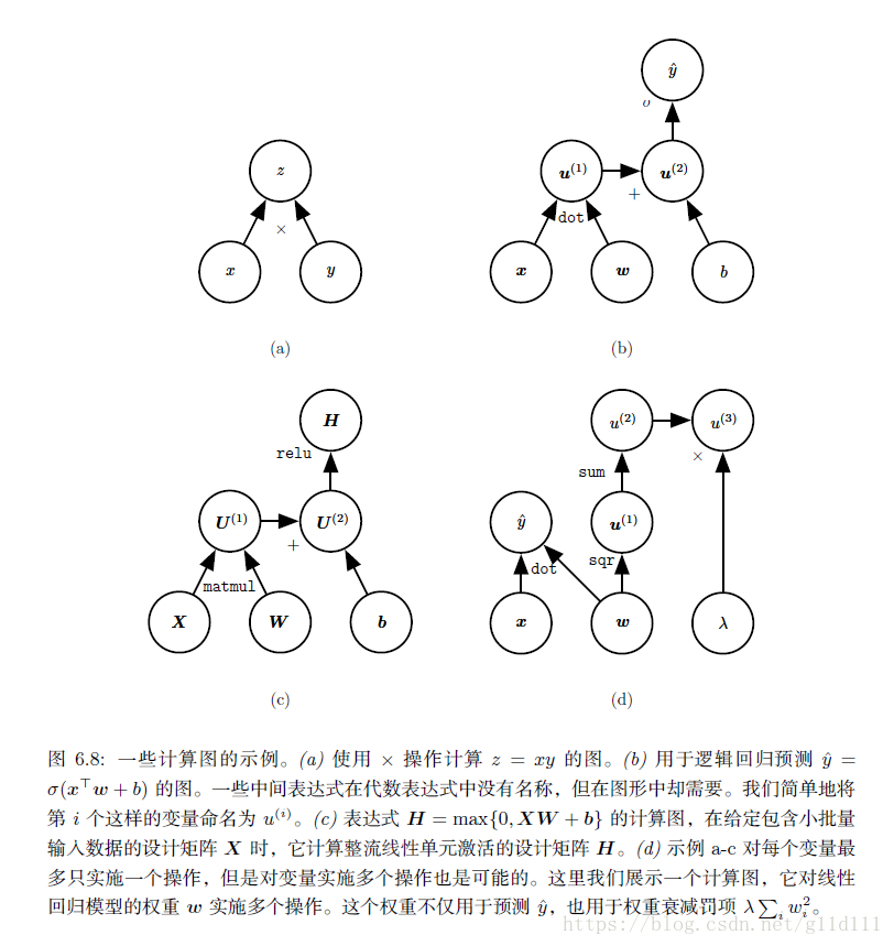
为了更精确地描述反向传播算法，使用更精确的 计算图（computational graph）语言是很有帮助的。将计算抽象为图形的方法有很多，这里，我们使用图中的每一个节点来表示一个变量（可以是标量、向量、矩阵、张量等各种形式）。
为了形式化我们的图形，我们还需引入 算子（operator）这一概念（PyTorch、Tensorflow等框架提供了成百上千种不同的算子，比如卷积、Pooling、GRU、LSTM、RNN等等等等）。算子（operator是指一个或多个变量的简单函数（也可能不那么“简单”)。我们的图形语言伴随着一组被允许的操作。我们可以通过将多个操作复合在一起来描述更为复杂的函数。
这里，假设每个算子只返回单个输出变量。目的是：避免引入对概念理解不重要的许多额外细节。

注意，如果一个变量y是由变量x经过一个**算子(operator)**得到的，那么在计算图中，会建立一条从x到y的有向边。

而每个节点的名称，在一般的框架中，是用op的名称表示（加上一些参数，比如conv的话，会加上kernel size， stride等参数）
下图[2]就是计算图的实例：

在这里插入图片描述

2.2 `Symbol2Symbol`

计算图说完了，下面说说以PyTorch为代表的动态图和以Tensorflow、Theano为代表的静态图的差别。这里面就不得不提到这个Symbol2Symbol了。

代数表达式和计算图都对符号(symbol) 或不具有特定值的变量进行操作。这些代数或者基于图的表达式被称为符号表示(symbolic representation)。
这个部分很好理解，因为我们对网络的输入每个batch、每个样本的的内容都不一样，为了避免重复的计算（比如重复的求解梯度表达式），所以需要制定出每个算子(operator)的确定的计算逻辑。

当我们实际使用或者训练神经网络时，我们必须给这些符号赋值。我们用一个特定的数值(numeric value) 来替代网络的符号输入x，例如 $[1.2,3,765,−1.8]^T$ 。

一些反向传播的方法采用计算图和一组用于图的输入的数值，然后返回在这些输入值处的梯度的数值。这种方法称为Symbol2Value——符号到数值的微分方法。也就是PyTorch以及其前身Torch和Caffe所采用的方法。

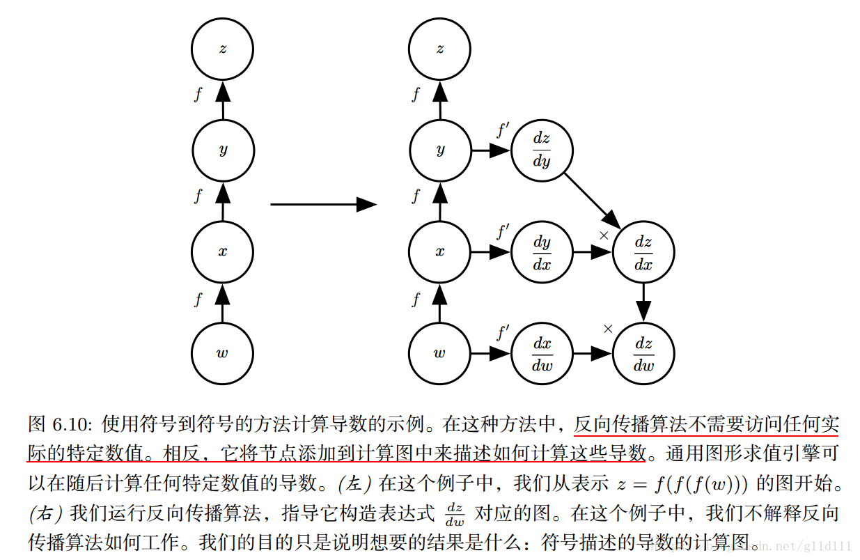
另一种方法是采用计算图和为计算图添加额外的节点（用于计算算子梯度），这些额外的节点提供了我们所需的导数的符号描述，称为Symbol2Symbol。这就是Theano和Tensorflow使用的方法。

Tensorflow和Theano类似，额外节点提供了所需导数的符号描述。这种方法的主要优点是导数可以使用与原始表达式相同的语言来描述。因为导数只是另外一张计算图(添加到主计算图中)，我们可以再次运行反向传播，对导数再进行求导就能得到更高阶的导数。

补充，这也就是为什么Tensorflow的模型在部署的时候，可以进行去掉训练节点这种方法的原因。

这也是Tensorflow这种静态图的优越之处————一劳永逸。DL这本书使用Symbol2Symbol来描述反向传播算法——为导数构建出一个计算图并加到主计算图中。

基于Symbol2Symbol——符号到符号的方法的描述包含了Symbol2Value符号到数值的方法。符号到数值的方法可以理解为执行了与符号到符号的方法中构建图的过程中完全相同的计算。关键的区别：符号到数值的方法不会显示出计算图。

下图是符号到符号的方法，即构建出导数的计算图，这里容易看出: $\frac {dz} {dw} = \frac {dx} {dw} * \frac {dz} {dx}$
$\frac {dz} {dx} = \frac {dy} {dx} * \frac {dz} {dy}$
在这里插入图片描述

3. 问题回顾

可能看到这里，大家觉得我只是罗列一些概念和知识点，并没有真正的回答开篇提到的问题“为什么在每次迭代（iteration）的时候，optimizer都要清空？”

这里结合前面提到的知识点进行总结可知：

PyTorch是动态图
动态图在每次iteration后都需要重建图本身
PyTorch的optimizer默认情况会自动对梯度进行accumulate[4]，所以对下一次iteration（一个新的batch），需要对optimizer进行清空操作。使用方式如下:

for epoch in range(2):  # loop over the dataset multiple times

    running_loss = 0.0
    for i, data in enumerate(trainloader, 0):
        # get the inputs
        inputs, labels = data

        # 情况参数梯度
        optimizer.zero_grad()

        # forward + backward + optimize
        outputs = net(inputs)
        loss = criterion(outputs, labels)
        loss.backward()
        optimizer.step()

        # print statistics
        running_loss += loss.item()
        if i % 2000 == 1999:    # print every 2000 mini-batches
            print('[%d, %5d] loss: %.3f' %
                  (epoch + 1, i + 1, running_loss / 2000))
            running_loss = 0.0

print('Finished Training')

[1] 《PyTorch学习笔记(11)——论nn.Conv2d中的反向传播实现过程》
[2] Autograd In PyTorch
[3] 《Deep Learning——6.5 反向传播与其它的微分算法》
[4] PyTorch 1.0.0.dev20181002 TRAINING A CLASSIFIER