1 前言
最近看了一些有关行人过街意图识别以及轨迹预测的论文,觉得这方面的研究还是比较有意思的,并且对交通领域的安全分析具有一定的研究价值,特此进行整理与解析。
这里,我们先简单了解一下何为过街意图识别以及轨迹预测。
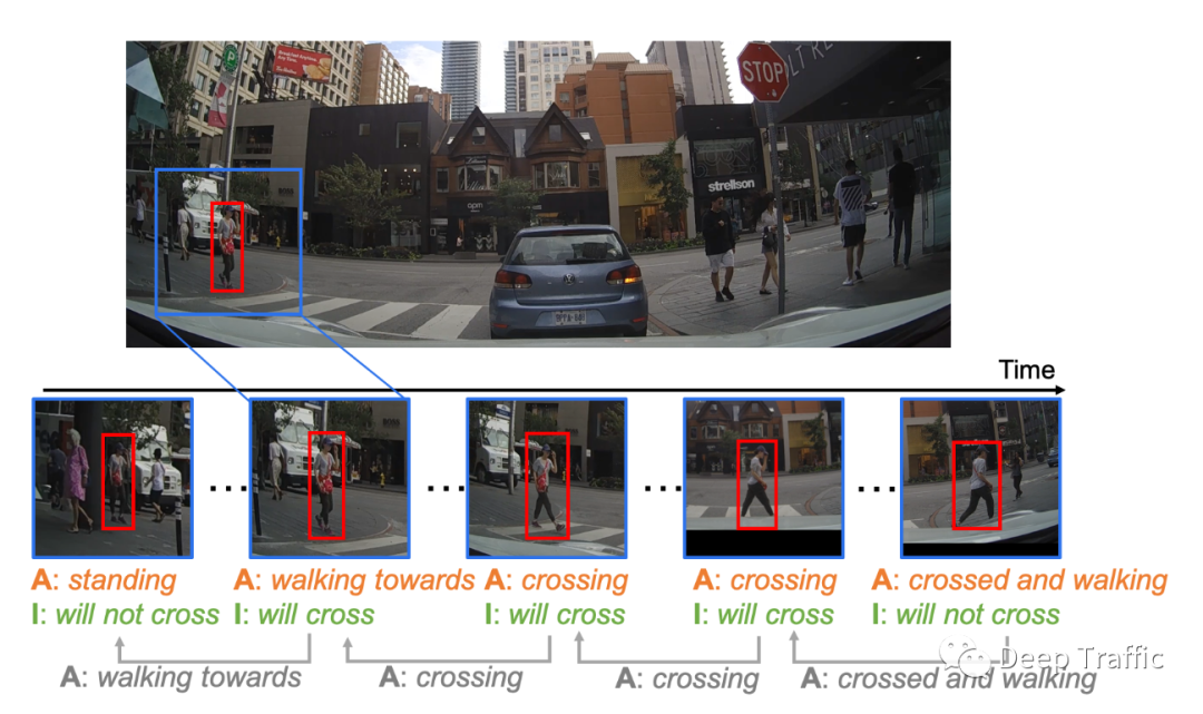
事实上,两个任务的输入具有一定的相似性,即都是通过观察一段时间的行人(车辆)历史帧,然后确定未来几秒内行人的过街意图(即是否过街的二分类问题)或者预测未来几秒内行人的运动轨迹。
因此,这两个任务对于自动驾驶、交通安全分析和事故阻止都有相当重要的意义。
写到这里,读者可以自行想象一下,过街意图识别以及轨迹预测与什么因素有关呢?
就过街意图而言,可能相关的因素有:行人历史的轨迹以及周围环境。事实上,行人历史轨迹一定程度上反映了行人本身的目的(想去哪儿,着急不着急等等),而环境因素是外在的限制,一定程度表明是否具备过街的条件。举个例子,你在过街的时候看见一辆车很快的靠近你,你还会坚持过街嘛?这显然不会,除非你头铁不怕死。与过街意图类似,轨迹预测也与行人历史的轨迹以及周围环境相关。
早期的一些研究中,因为环境信息的不易获取性,他们通常会忽略对周围环境因素的建模,比如在行人轨迹预测任务中,会忽略“行人-行人”之间的交互。显然,忽略这些环境因素大概率会预测不准。
可以想象,你日常走路过程中(特别是在拥挤的商场),你会关注周围其他人的位置、走向以及步速吗?答案是显然的,要不然别人该骂你“走路不长眼睛了”。

因此,在近期的一些研究中,同时考虑历史状态以及环境因素几乎是所以相关研究的标配了,所以后续的文章我们会探究这些研究里面的闪光点。
本文的解析对象为Social LSTM,是2016年的一篇CVPR,可以清晰地从作者名单中看到“Feifei Li”的字样,可见文章质量还是很高的。
这里我给出文章的链接以及代码链接:
文章链接:
“https://cvgl.stanford.edu/papers/CVPR16_Social_LSTM.pdf
代码链接:
“https://github.com/quancore/social-lstm
接下来,我们就结合原文和代码,以及网上其他大佬写的总结, 写一篇关于Social LSTM的解析。
2 论文解读
在这篇文章中,作者认为轨迹预测其实就是序列生成问题,而序列生成问题当时主流解决方法都从循环神经网络(如GRU或者LSTM)入手。所以本文作者就利用LSTM来才从行人的历史轨迹中学习行人的运动模式。
因为考虑到在一些稍微复杂/拥挤的场景中,行人和行人之间的轨迹是相互影响的,所以作者引入了“Social”(即人与人之间的交互)的概念,这也是“Social LSTM”中“Social”的来源。
为了去建立“Social”,本文的核心是:对于每个行人利用一个LSTM学习其运动模式,之后引入“Social pooling layer”使得空间相近的行人之间能够共享彼此的运动模式(即LSTM的隐藏状态)。
如下图所示,并以黑色轨迹为例,其周围的轨迹有蓝色和橙色两条轨迹,而红色轨迹不在其周围被排除。可见预测黑色轨迹时,除了黑色轨迹的当前时刻(T=1)LSTM隐藏状态外,蓝色轨迹和橙色轨迹的LSTM隐藏状态通过“Social pooling layer”聚合后也被一同输入到下一时刻(T=2)的LSTM中。
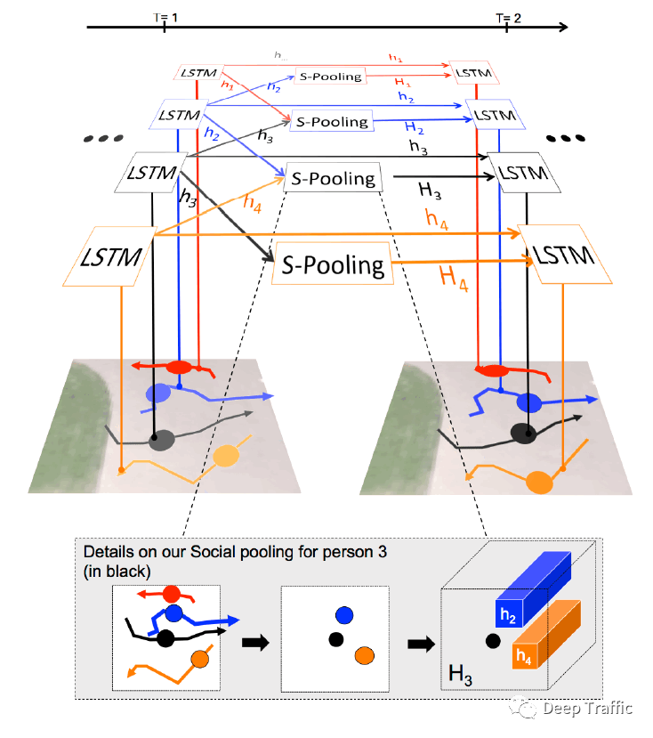
这样的操作其实并不难理解,但是具体关于“Social pooling layer”的运算细节,需要进一步解释说明。
(2.1)Social pooling layer
作者首先提到:
“every person has a different number of neighbors and in very dense crowds, this number could be prohibitively high.
即每个行人周围的行人数量可能是不等的,而且在一些拥堵的场景下,周围的数量可能非常多,而反观一些简单的场景,周围行人的数量可能较少。
为了克服这种被观测行人周围的行人数量不等的问题,作者引入了“Social pooling layer”,目的是将数量不等的周围行人的运动状态(隐藏在LSTM中)聚合成一个统一大小的张量/特征图,具体的实现方式如下图所示。
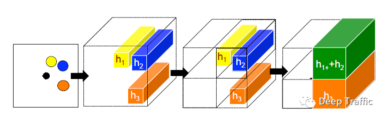
具体的操作可以分解为:
(1)确定邻节点:以被观察的行人的当前位置为中心(图中黑点),寻找其一定范围内的其他行人(即邻节点,图中的黄、蓝、橙点);
(2)隐藏状态嵌入:对于所有邻节点,获取其当前时刻通过LSTM后的隐藏状态,每个状态维度为;
(3)划分网格:将观察的邻近区域划分成一个的网格;
(4)隐藏状态聚合:将同属一个网格的邻节点的隐藏状态聚合,聚合聚合的方式就是简单的相加,最终获得一个的张量
更具体地,我们结合代码来看一下具体的实现:
def getGridMask(frame, dimensions, num_person, neighborhood_size, grid_size, is_occupancy = False):
    '''
    This function computes the binary mask that represents the
    occupancy of each ped in the other's grid
    params:
    frame : This will be a MNP x 3 matrix with each row being [pedID, x, y]
    dimensions : This will be a list [width, height]
    neighborhood_size : Scalar value representing the size of neighborhood considered
    grid_size : Scalar value representing the size of the grid discretization
    num_person : number of people exist in given frame
    is_occupancy: A flag using for calculation of accupancy map

    '''
    mnp = num_person

    width, height = dimensions[0], dimensions[1]
    if is_occupancy:
        frame_mask = np.zeros((mnp, grid_size**2))
    else:
        frame_mask = np.zeros((mnp, mnp, grid_size**2))
    frame_np =  frame.data.numpy()

    #width_bound, height_bound = (neighborhood_size/(width*1.0)), (neighborhood_size/(height*1.0))
    width_bound, height_bound = (neighborhood_size/(width*1.0))*2, (neighborhood_size/(height*1.0))*2
    #print("weight_bound: ", width_bound, "height_bound: ", height_bound)

    #instead of 2 inner loop, we check all possible 2-permutations which is 2 times faster.
    list_indices = list(range(0, mnp))
    for real_frame_index, other_real_frame_index in itertools.permutations(list_indices, 2):
        current_x, current_y = frame_np[real_frame_index, 0], frame_np[real_frame_index, 1]

        width_low, width_high = current_x - width_bound/2, current_x + width_bound/2
        height_low, height_high = current_y - height_bound/2, current_y + height_bound/2

        other_x, other_y = frame_np[other_real_frame_index, 0], frame_np[other_real_frame_index, 1]

        #if (other_x >= width_high).all() or (other_x < width_low).all() or (other_y >= height_high).all() or (other_y < height_low).all():
        if (other_x >= width_high) or (other_x < width_low) or (other_y >= height_high) or (other_y < height_low):
                # Ped not in surrounding, so binary mask should be zero
                #print("not surrounding")
                continue
        # If in surrounding, calculate the grid cell
        cell_x = int(np.floor(((other_x - width_low)/width_bound) * grid_size))
        cell_y = int(np.floor(((other_y - height_low)/height_bound) * grid_size))

        if cell_x >= grid_size or cell_x < 0 or cell_y >= grid_size or cell_y < 0:
                continue

        if is_occupancy:
            frame_mask[real_frame_index, cell_x + cell_y*grid_size] = 1
        else:
            # Other ped is in the corresponding grid cell of current ped
            frame_mask[real_frame_index, other_real_frame_index, cell_x + cell_y*grid_size] = 1


    return frame_mask
以上代码的核心在于作者建立一个frame_mask的矩阵,用来记录每个行人和他周围行人之间的位置关系。
其中作者利用如下代码来计算周围行人到被观察行人的相对位置(即cell_x和cell_y的)的:
cell_x = int(np.floor(((other_x - width_low)/width_bound) * grid_size))
cell_y = int(np.floor(((other_y - height_low)/height_bound) * grid_size))
获得了这样的frame_mask矩阵后,就需要对周围行人的隐藏状态进行聚合,其具体实现代码如下:
def getSocialTensor(self, grid, hidden_states):
    '''
    Computes the social tensor for a given grid mask and hidden states of all peds
    params:
    grid : Grid masks
    hidden_states : Hidden states of all peds
    '''
    # Number of peds
    numNodes = grid.size()[0]

    # Construct the variable
    social_tensor = Variable(torch.zeros(numNodes, self.grid_size*self.grid_size, self.rnn_size))
    if self.use_cuda:
        social_tensor = social_tensor.cuda()

    # For each ped
    for node in range(numNodes):
        # Compute the social tensor
        social_tensor[node] = torch.mm(torch.t(grid[node]), hidden_states)

    # Reshape the social tensor
    social_tensor = social_tensor.view(numNodes, self.grid_size*self.grid_size*self.rnn_size)
    return social_tensor
论文中,作者将网格划分和聚合的方式用以下公式表述:
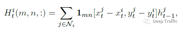
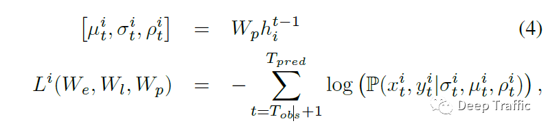
其中,函数表示周围行人是否在行人的范围内,而为行人前一时刻(即)的LSTM隐藏层状态。
很明显,两者用了简单的相乘后求和的方式进行了隐藏状态的聚合。在上述代码中,作者利用
torch.mm(torch.t(grid[node]), hidden_states)实现相乘和求和。
(2.2)Social LSTM
在上面,我们根据代码解析了Social Pooling层内部具体的运算机制,接下来,我们来探讨Social LSTM的具体运算。
在之前的一篇知乎文章(https://zhuanlan.zhihu.com/p/342149300)中,已经有大佬画了一个大致的运算步骤图,我补充他缺少的部分,重新绘制了如下的运算流程图。
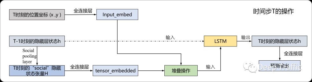
具体实现代码如下所示:
# Compute the social tensor
social_tensor = self.getSocialTensor(grid_current, hidden_states_current)

# Embed inputs
input_embedded = self.dropout(self.relu(self.input_embedding_layer(nodes_current)))
# Embed the social tensor
tensor_embedded = self.dropout(self.relu(self.tensor_embedding_layer(social_tensor)))

# Concat input
concat_embedded = torch.cat((input_embedded, tensor_embedded), 1)

if not self.gru:
    # One-step of the LSTM
    h_nodes, c_nodes = self.cell(concat_embedded, (hidden_states_current, cell_states_current))
else:
    h_nodes = self.cell(concat_embedded, (hidden_states_current))


# Compute the output
outputs[framenum*numNodes + corr_index.data] = self.output_layer(h_nodes)
结合上图和上面的代码,可见流程图和代码实现一一对应,这里的函数(self.input_embedding_layer,self.tensor_embedding_layer以及self.output_layer)均为全连接运算,我们就不过多赘述了。
(2.3)损失函数
原文中,作者提到利用时刻的LSTM隐藏层状态来预测时刻的轨迹位置分布。值得注意的是,这个轨迹分布被假设为二元正态分布,由五个参数确定,分别为和方向的均值和方差,以及协方差。
事实上,上图Social LSTM的运算流程图的预测输出就是每个行人的预测轨迹分布,维度为5。将这些预测的位置分布和ground truth拿过来计算损失函数(即negative log-Likelihood loss),损失函数定义为;
具体实现为:
def Gaussian2DLikelihood(outputs, targets, nodesPresent, look_up):
    '''
    params:
    outputs : predicted locations
    targets : true locations
    assumedNodesPresent : Nodes assumed to be present in each frame in the sequence
    nodesPresent : True nodes present in each frame in the sequence
    look_up : lookup table for determining which ped is in which array index

    '''
    seq_length = outputs.size()[0]
    # Extract mean, std devs and correlation
    mux, muy, sx, sy, corr = getCoef(outputs)

    # Compute factors
    normx = targets[:, :, 0] - mux
    normy = targets[:, :, 1] - muy
    sxsy = sx * sy

    z = (normx/sx)**2 + (normy/sy)**2 - 2*((corr*normx*normy)/sxsy)
    negRho = 1 - corr**2

    # Numerator
    result = torch.exp(-z/(2*negRho))
    # Normalization factor
    denom = 2 * np.pi * (sxsy * torch.sqrt(negRho))

    # Final PDF calculation
    result = result / denom

    # Numerical stability
    epsilon = 1e-20

    result = -torch.log(torch.clamp(result, min=epsilon))

    loss = 0
    counter = 0

    for framenum in range(seq_length):

        nodeIDs = nodesPresent[framenum]
        nodeIDs = [int(nodeID) for nodeID in nodeIDs]

        for nodeID in nodeIDs:
            nodeID = look_up[nodeID]
            loss = loss + result[framenum, nodeID]
            counter = counter + 1

    if counter != 0:
        return loss / counter
    else:
        return loss
(2.4)轨迹预测
轨迹预测预测的不仅仅是下一时刻的位置,而可能是未来一段时间内的位置序列。那么在观察了帧后,如何预测未来到的轨迹呢?
具体地,作者提到:
“During test time, we use the trained Social-LSTM models to predict the future position of the person. From time to , we use the predicted position from the previous Social-LSTM cell in place of the true coordinates in Eq. 2. The predicted positions are also used to replace the actual coordinates while constructing the Social hiddenstate tensor in Eq. 1 or the occupancy map in Eq.5.
也就是作者将当前时刻预测的位置作为下一时刻预测的输入来实现未来一段时间的位置预测。具体代码实现如下所示:
for tstep in range(args.obs_length-1, args.pred_length + args.obs_length-1):
    # Do a forward prop
    if grid is None: #vanilla lstm
        outputs, hidden_states, cell_states = net(ret_x_seq[tstep].view(1, numx_seq, 2), hidden_states, cell_states, [true_Pedlist[tstep]], [num_pedlist[tstep]], dataloader, look_up)
    else:
        outputs, hidden_states, cell_states = net(ret_x_seq[tstep].view(1, numx_seq, 2), [prev_grid], hidden_states, cell_states, [true_Pedlist[tstep]], [num_pedlist[tstep]], dataloader, look_up)

    # Extract the mean, std and corr of the bivariate Gaussian
    mux, muy, sx, sy, corr = getCoef(outputs)
    # Sample from the bivariate Gaussian
    next_x, next_y = sample_gaussian_2d(mux.data, muy.data, sx.data, sy.data, corr.data, true_Pedlist[tstep], look_up)

    # Store the predicted position
    ret_x_seq[tstep + 1, :, 0] = next_x
    ret_x_seq[tstep + 1, :, 1] = next_y
3 总结
写到这里,有关的Social LSTM的解析就结束了。一些小的细节,因为时间和篇幅问题,我也不过多赘述了.
推荐阅读:

我的2022届互联网校招分享

我的2021总结

浅谈算法岗和开发岗的区别

互联网校招研发薪资汇总
2022届互联网求职现状,金9银10快变成铜9铁10!!

公众号:AI蜗牛车

保持谦逊、保持自律、保持进步

发送【蜗牛】获取一份《手把手AI项目》(AI蜗牛车著)
发送【1222】获取一份不错的leetcode刷题笔记

发送【AI四大名著】获取四本经典AI电子书