摘 要: 平面点集的三角剖分在数值分析以及图形领域,都是极为重要的一项预处理技术。作为一种广泛应用的三角剖分技术,Delaunay三角剖分通过最大化最小角确保接近与规则的三角网和唯一性。本文通过概述 Delaunay 三角剖分的原理,实现了一种增量的 Delaunay 三角剖分构造算法。实验在真实人脸特征点数据和模拟数据上进行,并分别在不同数据规模下进行测试,结果表明了实现算法的有效性。
关键词: Delaunay 三角剖分;Voronoi 图;Delaunay 图; 三角剖分
引言
在数学和计算几何中,对于一个给定一般位置的离散点集 P P P,其 Delaunay 三角剖分记为 D T ( P ) DT(P) DT(P),满足 P P P 中的任何点都不在 D T ( P ) DT(P) DT(P) 中的任何三角形的外接圆内。Delaunay 三角剖分是三角剖分中所有三角形最小角度的最大化,倾向于避免狭长的三角形出现。由于 Boris Delaunay 从 1934 年开始研究这个课题,因此这种三角剖分是以 Boris Delaunay 的名字进行命名。
对于同一直线上的一组点,不存在 Delaunay 三角剖分;同一圆上的四个或多个点,存在不唯一的 Delaunay 三角剖分。通过考虑外切球,Delaunay 三角剖分的概念可以扩展到三维和更高的维度上,对欧几里得距离以外的度量进行推广是可能的。然而,在这些情况下,Delaunay 三角剖分不能保证存在或唯一。
本文实现 Delaunay 三角剖分算法,实验验证了算法的有效性,并将用在人脸特征点数据的三角剖分上。
Delaunay 三角剖分
本节中,首先由 Voronoi 图的对偶图引入 Delaunay 图的定义,继而引出 Delaunay 三角剖分的定义以及探讨如何构建 Delaunay 三角剖分。
Voronoi 图
平面离散点集 P P P 的 Voronoi 图是平面的一个子区域划分,其中包含 n n n 个子区域,分别对应于 P P P 中的各个基点 p ∈ P p \in P p∈P 所对应的子区域,由平面上以 p p p 为最近基点的所有点组成。
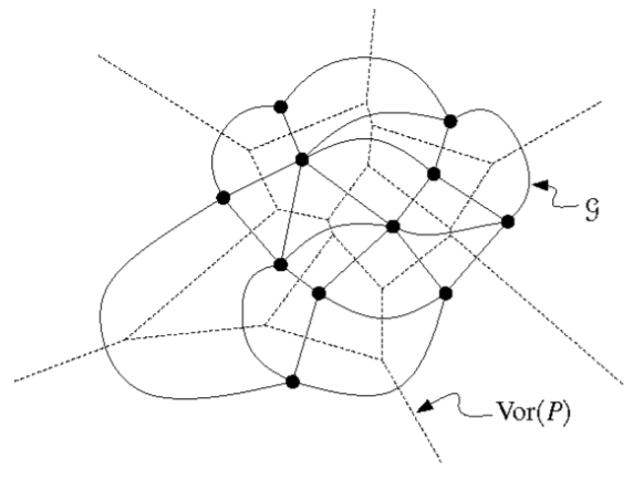
P P P 的 Voronoi 图,记作 V o r ( P ) Vor(P) Vor(P)。与基点 p p p 相对应的子区域,称为 p p p 的 Voronoi 单元,记作 V ( p ) V(p) V(p)。如 所示,本文主要研究 Voronoi 图的对偶图,记作 G G G。其中,对应于每一个 Voronoi 单元,各有一个节点,若两个单元之间公用一条边,则在这两个单元各自对应的节点之间,联接一条弧。因此,对应于 V o r ( P ) Vor(P) Vor(P) 中的每一条边, G G G 中都有一条弧与之对应。正如 所示,在 G G G 的所有有界面与 V o r ( P ) Vor(P) Vor(P) 中的所有顶点之间,存在一个一一对应关系。
Delaunay 图
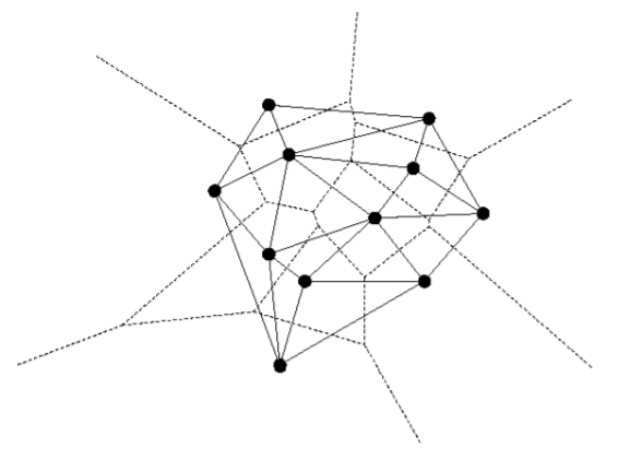
考察 G G G 的如下直线嵌入。其中,与 Voronoi 单元 V ( p ) V(p) V(p) 对应的节点,用点 p p p 来实现;而联接于 V ( p ) V(p) V(p) 和 V ( q ) V(q) V(q) 之间的弧,则用线段 p q ‾ \overline{pq} pq 来实现(如 下图 所示)。这一直线嵌入,称 作 P P P 的 Delaunay 图,记作 D G ( P ) DG(P) DG(P)。 点集的 Delaunay 图总是一个平面图,该直线嵌入中的任何两条边都不会相互跨越。
定理 1. 任何平面点集的 Delaunay 图都是一个平面图。
证明 1. 为证明这一结论,需要利用 Voronoi 图的一个特性,此处将借助 Delaunay 图的概念,进行具体证明。
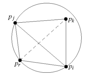
如 所示, p i p j ‾ \overline{p_ip_j} pipj 是 Delaunay 图 D G ( P ) DG(P) DG(P) 中的一条边,当且仅当存在这样一个闭圆盘 C i j C_{ij} Cij:它的边界经过 p i p_i pi 和 p j p_j pj,而且其中不包含来自 P P P 的任何其它基点。
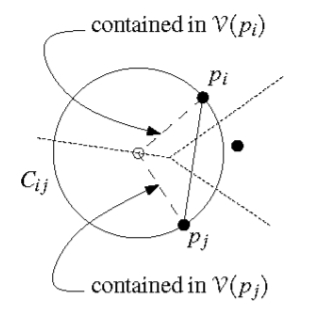
由顶点 p i p_i pi、 p j p_j pj 以及 C i j C_{ij} Cij 的中心确定的那个三角形,记作 t i j t_{ij} tij。可以看出, t i j t_{ij} tij 的联接于 p i p_i pi 和圆心 C i j C_{ij} Cij 之间那条边,必然完全落在 V ( p i ) V(p_i) V(pi) 内; p j p_j pj 也有类似的性质。现在,任取 D G ( P ) DG(P) DG(P) 中的另一条边 p k p l ‾ \overline{p_kp_l} pkpl,参照 C i j C_{ij} Cij 和 t i j t_{ij} tij 的定义方法,也可以定义出圆盘 C k l C_{kl} Ckl 以及三角形 t k l t_{kl} tkl。
若本定理不成立,即 p i p j ‾ \overline{p_ip_j} pipj 与 p k p l ‾ \overline{p_kp_l} pkpl 相交。既然 p k p_k pk 和 p l p_l pl 必然都落在圆盘 C i j C_{ij} Cij 之外,故必然也落在三角形 t i j t_{ij} tij 之外。这就意味着,在围成 t i j t_{ij} tij 的三条边中,与 C i j C_{ij} Cij 的圆心相关联的那两条边必有其一与 p k p l ‾ \overline{p_kp_l} pkpl 相交。同理,在围成 t k l t_{kl} tkl 的三条边中,与 C k l C_{kl} Ckl 的圆心相关联的那两条边也必有其一与 p i p j ‾ \overline{p_ip_j} pipj 相交。于是,若考虑在 t i j t_{ij} tij 的边界上、与 C i j C_{ij} Cij 的圆心相关联的那两条边,以及在 t k l t_{kl} tkl 的边界上、 与 C k l C_{kl} Ckl 的圆心相关联的那两条边,则前两条边中的某一条必然与后两条边中的某一条相交。然而,这种情况是不可能的,因为这两条边必然分别完全落在两个不同的 Voronoi 单元之内。 ◻
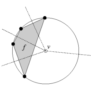
平面点集 P P P 的 Delaunay 图,是 Voronoi 图的对偶图的一个直线嵌入。正如我们在此前已经注意到的, V o r ( P ) Vor(P) Vor(P) 中的每个顶点,都分别对应于 Delaunay 图中的某张面。而在 Delaunay 图中围成每张面的各边,分别对应于 Voronoi 图中与某个 Voronoi 顶点相关联的各条 Voronoi 边(如 所示)。具体而言,在 Vor§ 中,若基点 p 1 , p 2 , p 3 , ⋯ , p k p_1, p_2, p_3, \cdots, p_k p1,p2,p3,⋯,pk 各自对应的(共 k k k 个)Voronoi 单元有一个共同的顶点 v v v,则在 D G ( P ) DG(P) DG(P) 中,与 v v v 相对应的面 f f f 的各个顶点,必然就是 p 1 , p 2 , p 3 , ⋯ , p k p_1, p_2, p_3, \cdots, p_k p1,p2,p3,⋯,pk。在这种情况下,点 p 1 , p 2 , p 3 , ⋯ , p k p_1, p_2, p_3, \cdots, p_k p1,p2,p3,⋯,pk 必然散落在某个以 v v v 为中心的圆周上。因此可以看出, f f f 不仅是一个 k k k-多边形,而且它必然还是凸的。
如果 P P P 中各点是随机分布的,任何四点恰好共圆的可能性就会很小。任何集合,只要其中没有任何四点共圆,我们就称它是处于一般性位置的。若 P P P 的确处于 一般性位置,则在其对应的 Voronoi 图中,每个顶点的度数必然都是 3。于是, D G ( P ) DG(P) DG(P)中的每一张有界面都必然是三角形。我们之所以经常将 D G ( P ) DG(P) DG(P) 称作 Delaunay 三角剖分(Delaunay triangulation),原因正在于此。然而,在此我们还是应该更为谨慎一些,姑且将 D G ( P ) DG(P) DG(P) 称作 P P P 的 Delaunay 图(Delaunay graph)。至于 Delaunay 三角剖分,我们对其有另一番定义:以 Delaunay 图为基础,通过引入联边 而得到的一个三角剖分。既然 D G ( P ) DG(P) DG(P) 中的每张面都是一个凸集,这样一个三角剖 分就可以很容易地得到。需要注意的是, P P P 的 Delaunay 三角剖分是唯一确定的,当且仅当 D G ( P ) DG(P) DG(P) 本身已经是一个三角剖分,换言之, P P P 是处于一般性位置的。
可以借助 Delaunay 图的概念,对关于 Voronoi 图有如下定理:
定理 2. 设 P P P 为任一平面点集,则在 P P P 的 Delaunay 图中:
- 三个点 p i , p j , p k ∈ P p_i, p_j, p_k \in P pi,pj,pk∈P 同为某张面的顶点,当且仅当 p i , p j , p k p_i, p_j, p_k pi,pj,pk 外接圆的内部不含 P P P 中的任何点;
- 两个点 p i , p j ∈ P p_i, p_j \in P pi,pj∈P 同时与某条边相关联,当且仅当存在一个闭圆盘 C C C,除了 p i p_i pi 和 p j p_j pj 落在其边界上之外,该圆盘不包含 P P P 中其它的任何点。
证明 2. 证明略,详见参考文献 [@cgaa_book] 定理 7.4。 ◻
同时,可以对 定理 1 重新表述为:
定理 3. 设 P P P 为平面上的任一点集,而 T T T 为 P P P 的任一三角剖分。则 T T T 是 P P P 的 Delaunay 三角剖分,当且仅当在 T T T 中每个三角形的外接圆的内部,都不包含 P P P 中的任何点。
证明 3 证明同 定理 1。 ◻
合法三角剖分
针对 P P P 的任一三角剖分 T T T,我们来考察其中的某一条边 e = p i p j ‾ e = \overline{p_ip_j} e=pipj。如果边 e e e 不属于 T T T 中那张无界面的边界,它必然会同时与两个三角形 △ p i p j p k \triangle p_ip_jp_k △pipjpk 和 △ p i p j p l \triangle p_ip_jp_l △pipjpl 相关联。如果这两个三角形合起来构成一个凸四边形,那么只要将 p i p j ‾ \overline{p_ip_j} pipj 从 T T T 中删去,代之以 p k p l p_kp_l pkpl,我们就可以得到另一个三角剖分 T ′ T' T′。如下图所示,这一操作称作边翻转(edge flip)。
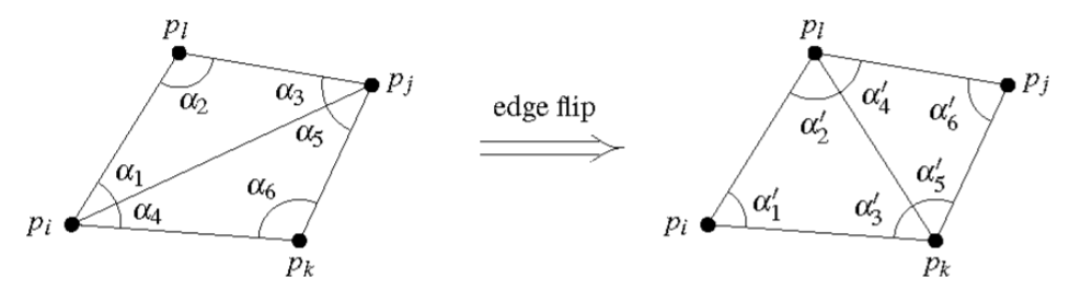
对比 T T T 与 T ′ T' T′ 的角度向量,共有六处不同: A ( T ) A(T) A(T) 中的六个角度 α 1 , α 2 , ⋯ , α 6 {\alpha_1, \alpha_2, \cdots, \alpha_6} α1,α2,⋯,α6,在 A ( T ′ ) A(T') A(T′) 中被换成了 α 1 ′ , α 2 ′ , ⋯ , α 6 ′ {\alpha'_1, \alpha'_2, \cdots, \alpha'_6} α1′,α2′,⋯,α6′。如果
KaTeX parse error: No such environment: equation* at position 8: \begin{̲e̲q̲u̲a̲t̲i̲o̲n̲*̲}̲ \min_{1 \leq i…
则将 e = p i p j ‾ e = \overline{p_ip_j} e=pipj 称作一条非法边(illegal edge)。换而言之,只要在对某条边进行边翻转操作之后,我们能够使局部的(即对应的六个角度中的)最小角增大,它就必然是一条非法边。由非法边的定义,可以立即得出如下观察结论。
推论 1. 设 e e e 为三角剖分 T T T 中的一条非法边。在 T T T 中对 e e e 进行边翻转操作之后,设新的三角剖分为 T ′ T' T′,则必有 A ( T ′ ) > A ( T ) A(T') > A(T) A(T′)>A(T)。
不含任何非法边的三角剖分,称作合法三角剖分(legal triangulation)。由上面的观察结论可知,角度最优的三角剖分必然也是合法三角剖分。
为了得到好的三角剖分,也就是要使其对应的角度向量尽可能地大。由合法三角剖分,引入对 Delaunay 三角剖分的角度向量的考察。
定理 4. 设 P P P 为平面上的任一点集。则 T T T 是 P P P 的一个合法三角剖分,当且仅当 T T T 是 P P P 的 Delaunay 三角剖分。
证明 4. 证明略,详见参考文献 [@cgaa_book; @dengjunhui] 定理 9.8。 ◻
既然任一角度最优的三角剖分都必合法,故由 可得出推论: P P P 的任一角度最优的三 角剖分,必是P的一个 Delaunay 三角剖分。当P处于一般性位置时,合法三角剖分是唯一存在的。它就是唯一的那个角度最优的三角剖分,即与 Delaunay 图完全吻合的那个唯一的 Delaunay 三角剖分。
可以证明,在 P P P 的所有三角剖分中,Delaunay 三角剖分使最小角达到最大。 P P P 的任一角度最优的三角剖分,必是 P P P 的一个 Delaunay 三角剖分。
构造 Delaunay 三角剖分
P P P 的 Delaunay 三角剖分的确是一种适宜的三角剖分。其原因在于,Delaunay 三角剖分可使其中的最小角最大化。本节中,主要介绍采用随机增量式算法来直接计算 Delaunay 三角剖分。
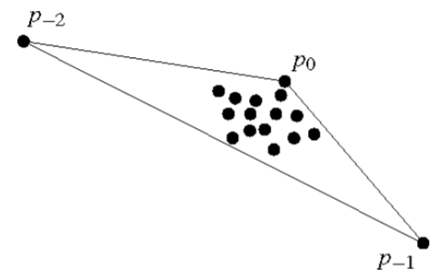
首先用一个足够大的三角形将整个点集 P P P 包围起来,需要引入两个辅助点 p − 1 p_{-1} p−1 和 p − 2 p_{-2} p−2,它们与 P P P 中的最高点联合构成的三角形,将包含所有的点。于是,我们需要构造 { p − 1 , p − 2 } ∪ P \{p_{-1}, p_{-2}\} \cup P { p−1,p−2}∪P 的三角剖分,在得到的三角剖分中只需要删除 p − 1 p_{-1} p−1 和 p − 2 p_{-2} p−2 以及与它们关联的各边即为 P P P 的三角剖分。为此,我们所选择的 p − 1 p_{-1} p−1 和 p − 2 p_{-2} p−2 必须相距足够远,才不致于对 P P P 的 Delaunay 三角剖分中的任何三角形有所影响。尤其必须保证的一点是,它们不能落在 P P P 中任何三点的外接圆内。
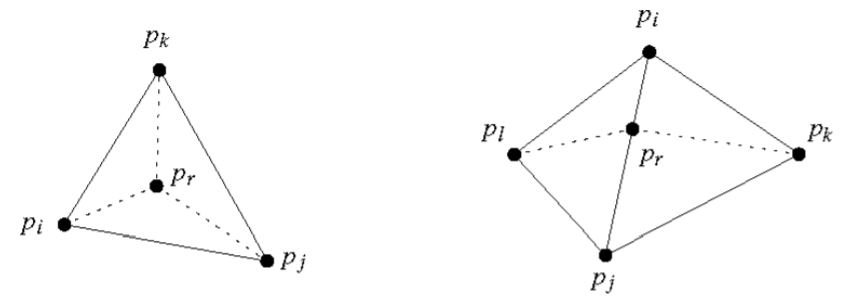
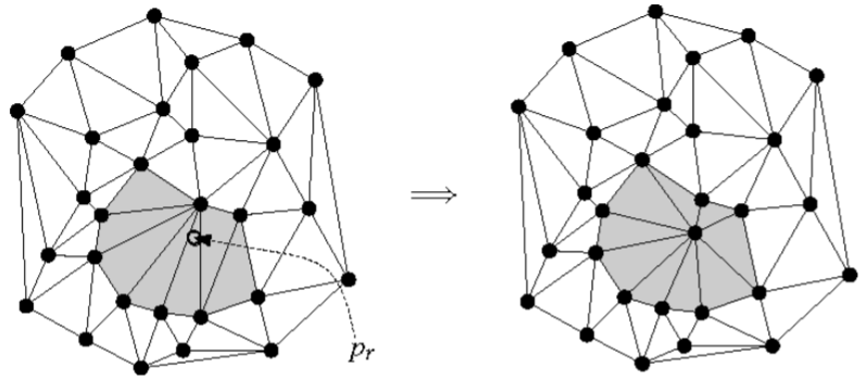
按随机次序逐一引入各点,整个过程中,都要维护并更新一个与当前点集对应的 Delaunay 三角剖分。考虑引入点 p r p_r pr 时的情况,如图所示。首先,要在当前的三角剖分中,确定 p r p_r pr落在哪个三角形内。然后,将 p r p_r pr 与该三角形的三个顶点分别联接起来,生 成三条边。倘若 p r p_r pr 碰巧落在三角剖分的某条边 e e e 上,就需要找到与 e e e 关联的那两个三角形,然后将 p r p_r pr 与对顶的那两个顶点分别联接起来,生成两条边。
这样,就得到了一个三角剖分,但它不一定是一个 Delaunay
三角剖分。因为,在引入点 p r p_r pr 之后,原来的某些边可能不再合法。为消除这些不合法性,需要针对每一条可能的非法边,调用一次子函数 LEGALIZEEDGE。这个子函数通过边翻转操作,将所有的非法边转换为合法边。为便于分析,不妨假定集合
P P P 由 ( n + 1 ) (n+1) (n+1) 个点组成。
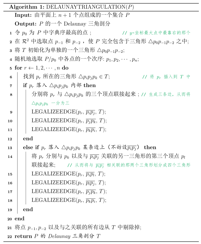
令 p 0 p_0 p0 为 P P P 中字典序最高的点 在 R 2 \mathcal{R}^2 R2 中选取点 p − 1 p_{-1} p−1 和 p − 2 p_{-2} p−2 ,使 P P P 完全包含于三角形 △ p 0 p − 1 p − 2 \triangle p_0p_{-1}p_{-2} △p0p−1p−2 之中将 T T T 初始化为单独的一个三角形 △ p 0 p − 1 p − 2 \triangle p_0p_{-1}p_{-2} △p0p−1p−2 随机地选取 P / p 0 P/{p_0} P/p0 中各点的一个次序: p 1 , p 2 , ⋯ , p n p_1, p_2, \cdots, p_n p1,p2,⋯,pn 将点 p − 1 , p − 2 p_{-1}, p_{-2} p−1,p−2 以及与之关联的所有边从 T T T 中剔除掉。
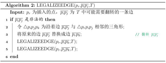
由 定理 2 可知,一个三角剖分是 Delaunay 三角剖分,当且仅当其中的所有边都是合法的。按照算法 LEGALTRIANGULATION 的原则,不断地对非法边实施翻转操作,直到重新回到一个合法三角剖分。由于原来的任何一条合法边 p i p j ‾ \overline{p_ip_j} pipj,只有在与其相关联的三角形发生变化时,才有可能会成为一条非法边。因此,我们只需检查新生成的那些三角形的各边。这项工作是由子程序 LEGALIZEEDGE 来完成的,它会对有关的各边进行检查,若有必要,则进行边翻转。每翻转一条边之后,可能又会进而使得其它的某些边变得非法。对于所有可能的新非法边,LEGALIZEEDGE 都要递归地调用自己,逐一进行核查。
其中, 第 2 行要检查某条边的合法性。从 LEGALIZEEDGE的代码可以清楚地看出,由于 p r p_r pr 的插入而新生出来的每一条边, 都必然与 p r p_r pr 相关联。这一点也可以从中看出:在原有的某些三角形被销毁之后,新生出来的三角形用灰色表示。任何一条边若(从合法)变成非法,则与之相关联的(至多两个)三角形中必有其一发生了变化。所有可能变为非法的边,都必然会接受该算法的检查。也就是说,该算法是正确的。需要指出的是:该算法也不致于陷入无限的死循环。这是因为每经过一次翻转,三角剖分的角度向量总是会单调地增长。
实验与结果
本节中,主要通过使用 Python 程序实现 Delaunay 三角剖分算法,通过仿真实验验证了算法的有效性。
实验环境
实验在配置为 Intel® Core™ 7-10510U CPU @ 1.80GHz.2.30 GHz 和 16 GB memory 的笔记本上使用 Python 3.7 进行。
结果与分析
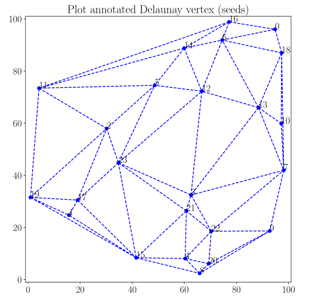
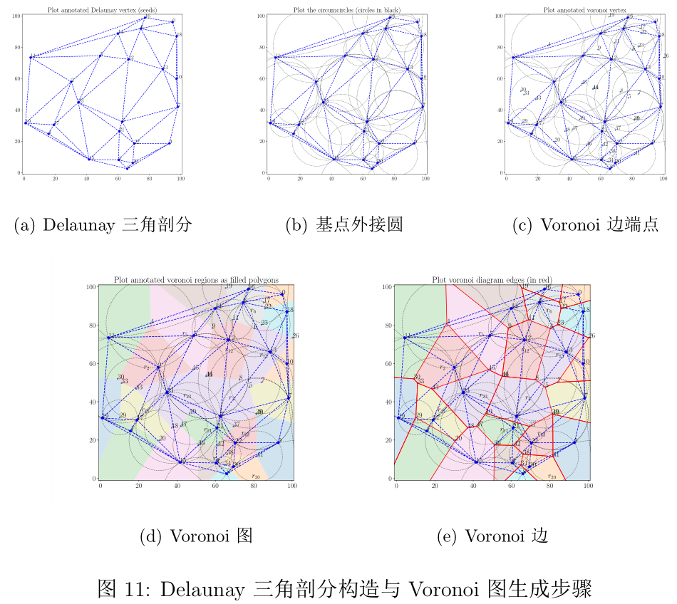
为了方便显示, 展示了 24 个点的 Delaunay 三角剖分构造与 Voronoi 图生成步骤的可视化结果。关于完整的生成步骤视频,详见支撑材料。
Delaunay 三角剖分可视化
首先,随机生成包括若干点的集合 P P P,采用 依次迭代,最终生成 P P P 的一个三角剖分。为了可视化方便,设置点集 P P P 的大小为 24,生成的三角剖分如 所示。
给出了人脸部特征点的三角剖分实例, 是 Trump 脸部原图, 是对其脸部 68 个特征点的 Delaunay 三角剖分。

Voronoi 图可视化
在 Delaunay 三角剖分的基础上,构造 Voronoi
图。作每一个三角面的外接圆(如 ),这些外接圆的圆心即为 Voronoi 图各边的端点(如 )。连接同一 Delaunay 边为弦的两个外接圆圆心形成 Voronoi 图的各边,分别将 Voronoi 图各个子区域涂色如 和 所示。
算法运行时间
为了统计数据规模对算法运行时间的影响,分别生成 10、100、1000 的基点进行实验,Delaunay 三角剖分算法运行时间实验结果如下表所示。由此可见,随着数据规模的增加,算法运行时间对数线性增加。可以证明,的时间复杂度为 O ( n log n ) \mathcal{O}(n \log n) O(nlogn)。
   \#     基点规模   Delaunay 三角面数量   运行时间 (s)

----- ---------- --------------------- --------------

   $1$          10                    13         0.0049
   $2$         100                   186         0.9200
   $3$        1000                  1977         6.1894
   $4$       10000                 19964       560.1147

  : Delaunay 三角剖分算法运行时间
另外, 也报告了不同规模基点 Delaney 三角剖分生成三角网格的数目。可以证明, 由 算法1 生成的三角形,总数目的期望值不超过 9 n + 1 9n + 1 9n+1。
小结
本文概述了 Delaunay 三角剖分的原理,详细阐述了构建 Delaunay 三角剖分的算法。分别在模拟数据和真实数据上进行了实验验证,实验结果表明算法的有效性。
参考资料
[1] M. de Berg, O. Cheong, M. van Kreveld, and M. Overmars, Computational
Geometry: Algorithms and Applications, 2008.
[2] 邓俊辉, 计算几何算法与应用 (中文版), 2011.
[3] https://github.com/jmespadero/pyDelaunay2D
[4] https://blog.csdn.net/weixin_42512684/article/details/106650061
附录
主要程序
# -*- coding: ascii -*-
"""
Simple structured Delaunay triangulation in 2D with Bowyer-Watson algorithm.

Written by Jose M. Espadero ( http://github.com/jmespadero/pyDelaunay2D )
Based on code from Ayron Catteau. Published at http://github.com/ayron/delaunay

Just pretend to be simple and didactic. The only requisite is numpy.
Robust checks disabled by default. May not work in degenerate set of points.
"""

import numpy as np
from math import sqrt


class Delaunay2D:
    """
    Class to compute a Delaunay triangulation in 2D
    ref: http://en.wikipedia.org/wiki/Bowyer-Watson_algorithm
    ref: http://www.geom.uiuc.edu/~samuelp/del_project.html
    """

    def __init__(self, center=(0, 0), radius=9999):
        """ Init and create a new frame to contain the triangulation
        center -- Optional position for the center of the frame. Default (0,0)
        radius -- Optional distance from corners to the center.
        """
        center = np.asarray(center)
        # Create coordinates for the corners of the frame
        self.coords = [center+radius*np.array((-1, -1)),
                       center+radius*np.array((+1, -1)),
                       center+radius*np.array((+1, +1)),
                       center+radius*np.array((-1, +1))]

        # Create two dicts to store triangle neighbours and circumcircles.
        self.triangles = {

    }
        self.circles = {

    }

        # Create two CCW triangles for the frame
        T1 = (0, 1, 3)
        T2 = (2, 3, 1)
        self.triangles[T1] = [T2, None, None]
        self.triangles[T2] = [T1, None, None]

        # Compute circumcenters and circumradius for each triangle
        for t in self.triangles:
            self.circles[t] = self.circumcenter(t)

    def circumcenter(self, tri):
        """Compute circumcenter and circumradius of a triangle in 2D.
        Uses an extension of the method described here:
        http://www.ics.uci.edu/~eppstein/junkyard/circumcenter.html
        """
        pts = np.asarray([self.coords[v] for v in tri])
        pts2 = np.dot(pts, pts.T)
        A = np.bmat([[2 * pts2, [[1],
                                 [1],
                                 [1]]],
                      [[[1, 1, 1, 0]]]])

        b = np.hstack((np.sum(pts * pts, axis=1), [1]))
        x = np.linalg.solve(A, b)
        bary_coords = x[:-1]
        center = np.dot(bary_coords, pts)

        # radius = np.linalg.norm(pts[0] - center) # euclidean distance
        radius = np.sum(np.square(pts[0] - center))  # squared distance
        return (center, radius)

    def inCircleFast(self, tri, p):
        """Check if point p is inside of precomputed circumcircle of tri.
        """
        center, radius = self.circles[tri]
        return np.sum(np.square(center - p)) <= radius

    def inCircleRobust(self, tri, p):
        """Check if point p is inside of circumcircle around the triangle tri.
        This is a robust predicate, slower than compare distance to centers
        ref: http://www.cs.cmu.edu/~quake/robust.html
        """
        m1 = np.asarray([self.coords[v] - p for v in tri])
        m2 = np.sum(np.square(m1), axis=1).reshape((3, 1))
        m = np.hstack((m1, m2))    # The 3x3 matrix to check
        return np.linalg.det(m) <= 0

    def addPoint(self, p):
        """Add a point to the current DT, and refine it using Bowyer-Watson.
        """
        p = np.asarray(p)
        idx = len(self.coords)
        # print("coords[", idx,"] ->",p)
        self.coords.append(p)

        # Search the triangle(s) whose circumcircle contains p
        bad_triangles = []
        for T in self.triangles:
            # Choose one method: inCircleRobust(T, p) or inCircleFast(T, p)
            if self.inCircleFast(T, p):
                bad_triangles.append(T)

        # Find the CCW boundary (star shape) of the bad triangles,
        # expressed as a list of edges (point pairs) and the opposite
        # triangle to each edge.
        boundary = []
        # Choose a "random" triangle and edge
        T = bad_triangles[0]
        edge = 0
        # get the opposite triangle of this edge
        while True:
            # Check if edge of triangle T is on the boundary...
            # if opposite triangle of this edge is external to the list
            tri_op = self.triangles[T][edge]
            if tri_op not in bad_triangles:
                # Insert edge and external triangle into boundary list
                boundary.append((T[(edge+1) % 3], T[(edge-1) % 3], tri_op))

                # Move to next CCW edge in this triangle
                edge = (edge + 1) % 3

                # Check if boundary is a closed loop
                if boundary[0][0] == boundary[-1][1]:
                    break
            else:
                # Move to next CCW edge in opposite triangle
                edge = (self.triangles[tri_op].index(T) + 1) % 3
                T = tri_op

        # Remove triangles too near of point p of our solution
        for T in bad_triangles:
            del self.triangles[T]
            del self.circles[T]

        # Retriangle the hole left by bad_triangles
        new_triangles = []
        for (e0, e1, tri_op) in boundary:
            # Create a new triangle using point p and edge extremes
            T = (idx, e0, e1)

            # Store circumcenter and circumradius of the triangle
            self.circles[T] = self.circumcenter(T)

            # Set opposite triangle of the edge as neighbour of T
            self.triangles[T] = [tri_op, None, None]

            # Try to set T as neighbour of the opposite triangle
            if tri_op:
                # search the neighbour of tri_op that use edge (e1, e0)
                for i, neigh in enumerate(self.triangles[tri_op]):
                    if neigh:
                        if e1 in neigh and e0 in neigh:
                            # change link to use our new triangle
                            self.triangles[tri_op][i] = T

            # Add triangle to a temporal list
            new_triangles.append(T)

        # Link the new triangles each another
        N = len(new_triangles)
        for i, T in enumerate(new_triangles):
            self.triangles[T][1] = new_triangles[(i+1) % N]   # next
            self.triangles[T][2] = new_triangles[(i-1) % N]   # previous

    def exportTriangles(self):
        """Export the current list of Delaunay triangles
        """
        # Filter out triangles with any vertex in the extended BBox
        return [(a-4, b-4, c-4)
                for (a, b, c) in self.triangles if a > 3 and b > 3 and c > 3]

    def exportCircles(self):
        """Export the circumcircles as a list of (center, radius)
        """
        # Remember to compute circumcircles if not done before
        # for t in self.triangles:
        #     self.circles[t] = self.circumcenter(t)

        # Filter out triangles with any vertex in the extended BBox
        # Do sqrt of radius before of return
        return [(self.circles[(a, b, c)][0], sqrt(self.circles[(a, b, c)][1]))
                for (a, b, c) in self.triangles if a > 3 and b > 3 and c > 3]

    def exportDT(self):
        """Export the current set of Delaunay coordinates and triangles.
        """
        # Filter out coordinates in the extended BBox
        coord = self.coords[4:]

        # Filter out triangles with any vertex in the extended BBox
        tris = [(a-4, b-4, c-4)
                for (a, b, c) in self.triangles if a > 3 and b > 3 and c > 3]
        return coord, tris

    def exportExtendedDT(self):
        """Export the Extended Delaunay Triangulation (with the frame vertex).
        """
        return self.coords, list(self.triangles)

    def exportVoronoiRegions(self):
        """Export coordinates and regions of Voronoi diagram as indexed data.
        """
        # Remember to compute circumcircles if not done before
        # for t in self.triangles:
        #     self.circles[t] = self.circumcenter(t)
        useVertex = {

    i: [] for i in range(len(self.coords))}
        vor_coors = []
        index = {

    }
        # Build a list of coordinates and one index per triangle/region
        for tidx, (a, b, c) in enumerate(sorted(self.triangles)):
            vor_coors.append(self.circles[(a, b, c)][0])
            # Insert triangle, rotating it so the key is the "last" vertex
            useVertex[a] += [(b, c, a)]
            useVertex[b] += [(c, a, b)]
            useVertex[c] += [(a, b, c)]
            # Set tidx as the index to use with this triangle
            index[(a, b, c)] = tidx
            index[(c, a, b)] = tidx
            index[(b, c, a)] = tidx

        # init regions per coordinate dictionary
        regions = {

    }
        # Sort each region in a coherent order, and substitude each triangle
        # by its index
        for i in range(4, len(self.coords)):
            v = useVertex[i][0][0]  # Get a vertex of a triangle
            r = []
            for _ in range(len(useVertex[i])):
                # Search the triangle beginning with vertex v
                t = [t for t in useVertex[i] if t[0] == v][0]
                r.append(index[t])  # Add the index of this triangle to region
                v = t[1]            # Choose the next vertex to search
            regions[i-4] = r        # Store region.

        return vor_coors, regions
人脸特征点提取
import dlib
import cv2

predictor_path  = "./shape_predictor_68_face_landmarks.dat"
png_path = "./trump.jpeg"

txt_path = "./points.txt"
f = open(txt_path,'w+')


detector = dlib.get_frontal_face_detector()
predicator = dlib.shape_predictor(predictor_path)
win = dlib.image_window()
img1 = cv2.imread(png_path)


dets = detector(img1, 1)
print("Number of faces detected : {}".format(len(dets)))
for k,d in enumerate(dets):
    print("Detection {}  left:{}  Top: {} Right {}  Bottom {}".format(
        k,d.left(),d.top(),d.right(),d.bottom()
    ))
    lanmarks = [[p.x,p.y] for p in predicator(img1,d).parts()]
    for idx,point in enumerate(lanmarks):
        f.write(str(point[0]))
        f.write("\t")
        f.write(str(point[1]))
        f.write('\n')
可视化程序
#!/usr/bin/env python3
import time
import numpy as np
from delaunay2D import Delaunay2D


def vis(dt):

    """
    Demostration of how to plot the data.
    """
    import matplotlib.pyplot as plt
    import matplotlib.tri
    import matplotlib.collections

    plt.rcParams['font.family'] = 'serif'
    plt.rcParams['font.size'] = 18
    plt.rcParams['text.usetex'] = True

    from matplotlib.animation import FFMpegWriter

    # Create a plot with matplotlib.pyplot
    # fig, ax = plt.subplots()
    # ax.margins(0.1)
    # ax.set_aspect('equal')
    # plt.axis([-1, radius+1, -1, radius+1])

    # made the video of result
    metadata = dict(title='Hand tremor cleaning result', artist='Matplotlib', comment='Paper showing!')
    writer = FFMpegWriter(fps=15, metadata=metadata)
    fig = plt.figure(figsize=(10, 9))
    fig.tight_layout()

    with writer.saving(fig=fig,
                       outfile="output-delaunay2D_%d.mp4" % numSeeds,
                       dpi=300):
        # plt.axis('off')
        ax = plt.subplot(111)
        # Plot a step-by-step triangulation
        # Starts from a new Delaunay2D frame
        dt2 = Delaunay2D(center, 50 * radius)
        for i, s in enumerate(seeds):
            print("Inserting seed", i, s)
            dt2.addPoint(s)
            if i > 1:
                ax.margins(0.1)
                ax.set_aspect('equal')
                ax.set_title("%d" % i)
                ax.axis([-1, radius + 1, -1, radius + 1])

                for i, v in enumerate(seeds):
                    plt.annotate(i, xy=v)  # Plot all seeds
                for t in dt2.exportTriangles():
                    polygon = [seeds[i] for i in t]  # Build polygon for each region
                    plt.fill(*zip(*polygon), fill=False, color="b")  # Plot filled polygon

            # ax.axis("off")
            writer.grab_frame()

        plt.clf()
        ax = plt.subplot(111)
        ax.margins(0.1)
        ax.set_aspect('equal')
        ax.axis([-1, radius + 1, -1, radius + 1])
        # Plot our Delaunay triangulation (plot in blue)
        cx, cy = zip(*seeds)
        dt_tris = dt.exportTriangles()
        ax.triplot(matplotlib.tri.Triangulation(cx, cy, dt_tris), 'bo--')

        print("Plot annotated Delaunay vertex (seeds)")
        # Plot annotated Delaunay vertex (seeds)
        for i, v in enumerate(seeds):
            ax.set_title("Plot annotated Delaunay vertex (seeds)")

            plt.annotate(i, xy=v)

            writer.grab_frame()

        # Dump plot to file
        plt.savefig('output-delaunay2D_Delaunay_vertex-%d.pdf' % numSeeds)

        # DEBUG: Use matplotlib to create a Delaunay triangulation (plot in green)
        # DEBUG: It should be equal to our result in dt_tris (plot in blue)
        # DEBUG: If boundary is diferent, try to increase the value of your margin
        # ax.triplot(matplotlib.tri.Triangulation(*zip(*seeds)), 'g--')

        # DEBUG: plot the extended triangulation (plot in red)
        # edt_coords, edt_tris = dt.exportExtendedDT()
        # edt_x, edt_y = zip(*edt_coords)
        # ax.triplot(matplotlib.tri.Triangulation(edt_x, edt_y, edt_tris), 'ro-.')

        print("Plot the circumcircles (circles in black)")
        # Plot the circumcircles (circles in black)
        for c, r in dt.exportCircles():
            ax.set_title("Plot the circumcircles (circles in black)")

            ax.add_artist(plt.Circle(c, r, color='k', fill=False, ls='dotted'))

            writer.grab_frame()

        # Dump plot to file
        plt.savefig('output-delaunay2D_circumcircles-%d.pdf' % numSeeds)

        # Build Voronoi diagram as a list of coordinates and regions
        vc, vr = dt.exportVoronoiRegions()

        print("Plot annotated voronoi vertex")
        # Plot annotated voronoi vertex
        plt.scatter([v[0] for v in vc], [v[1] for v in vc], marker='.')
        for i, v in enumerate(vc):
            ax.set_title("Plot annotated voronoi vertex")

            plt.annotate(i, xy=v)

            writer.grab_frame()

        # Dump plot to file
        plt.savefig('output-delaunay2D_voronoi_vertex-%d.pdf' % numSeeds)

        print("Plot annotated voronoi regions as filled polygons")
        # Plot annotated voronoi regions as filled polygons
        for r in vr:
            ax.set_title("Plot annotated voronoi regions as filled polygons")

            polygon = [vc[i] for i in vr[r]]  # Build polygon for each region
            plt.fill(*zip(*polygon), alpha=0.2)  # Plot filled polygon
            plt.annotate("$r_{%d}$" % r, xy=np.average(polygon, axis=0))

            writer.grab_frame()
        # Dump plot to file
        plt.savefig('output-delaunay2D_voronoi-%d.pdf' % numSeeds)

        print("Plot voronoi diagram edges (in red)")
        # Plot voronoi diagram edges (in red)
        for r in vr:
            ax.set_title("Plot voronoi diagram edges (in red)")

            polygon = [vc[i] for i in vr[r]]  # Build polygon for each region
            plt.plot(*zip(*polygon), color="red")  # Plot polygon edges in red

            writer.grab_frame()

        # Dump plot to file
        plt.savefig('output-delaunay2D_voronoi_edge-%d.pdf' % numSeeds)

        plt.show()
        plt.close()


if __name__ == '__main__':

    ###########################################################
    # Generate 'numSeeds' random seeds in a square of size 'radius'
    numSeeds = 10
    radius = 100
    seeds = radius * np.random.random((numSeeds, 2))
    print("seeds:\n", seeds)
    print("BBox Min:", np.amin(seeds, axis=0),
          "Bbox Max: ", np.amax(seeds, axis=0))

    """
    Compute our Delaunay triangulation of seeds.
    """
    # It is recommended to build a frame taylored for our data
    time_start = time.time()
    center = np.mean(seeds, axis=0)
    dt = Delaunay2D(center, 50 * radius)

    # Insert all seeds one by one
    for s in seeds:
        dt.addPoint(s)
    time_end = time.time()

    # Dump number of DT triangles
    print(len(dt.exportTriangles()), "Delaunay triangles | Time: ",
          time_end - time_start)

    # vis(dt)