Kaggle的Time Series课程代码

Linear Regression With Time Series

该系列记录了一家零售店 30 天内精装书的销售数量。请注意，我们有一列带有时间索引日期的精装观察。

import pandas as pd
df = pd.read_csv("../input/ts-course-data/book_sales.csv",
               index_col="Date",#指定某列为行索引，否则自动索引0, 1, .....
               parse_dates=["Date"],#parse_dates=[0,1,2,3,4] : 尝试解析0，1，2，3，4列为时间格式；
               ).drop("Paperback", axis=1)#删除列
df.head()#df.head(n):该方法用于查看dataframe数据表中开头n行的数据，若参数n未设置，即df.head()，则默认查看dataframe中前5行的数据。

时间步长特征是我们可以直接从时间索引中得出的特征。最基本的时间步长特征是时间虚拟变量，它从头到尾计算序列中的时间步长。

import numpy as np

df['Time'] = np.arange(len(df.index))#函数返回一个有终点和起点的固定步长的排列，如[1,2,3,4,5]，起点是1，终点是6，步长为1。

df.head()

然后，时间虚拟变量让我们将曲线拟合到时间图中的时间序列，其中时间形成 x 轴。

import matplotlib.pyplot as plt
import seaborn as sns
plt.style.use("seaborn-whitegrid")
plt.rc(
    "figure",
    autolayout=True,
    figsize=(11, 4),
    titlesize=18,
    titleweight='bold',
)
plt.rc(
    "axes",
    labelweight="bold",
    labelsize="large",
    titleweight="bold",
    titlesize=16,
    titlepad=10,
)
%config InlineBackend.figure_format = 'retina'#避免绘制模糊图像,JuypterNotebook中的默认绘图看起来有些模糊。

fig, ax = plt.subplots()
ax.plot('Time', 'Hardcover', data=df, color='0.75')
ax = sns.regplot(x='Time', y='Hardcover', data=df, ci=None, scatter_kws=dict(color='0.25'))
ax.set_title('Time Plot of Hardcover Sales');

为了制作滞后特征，我们改变了目标系列的观察结果，使它们看起来发生在较晚的时间。在这里，我们创建了一个 1 步滞后功能，尽管也可以进行多步移动。

df['Lag_1'] = df['Hardcover'].shift(1)#Pandas dataframe.shift()函数根据需要的周期数移动索引，并带有可选的时间频率。该函数采用称为周期的标量参数，该参数表示要在所需轴上进行的平移次数。
df = df.reindex(columns=['Hardcover', 'Lag_1'])#reindex重新构建索引

df.head()

因此，滞后特征让我们可以将曲线拟合到滞后图中，其中系列中的每个观察值都与前一个观察值相对应。

fig, ax = plt.subplots()
ax = sns.regplot(x='Lag_1', y='Hardcover', data=df, ci=None,                 
                 scatter_kws=dict(color='0.25'))#sns.regplot()：绘图数据和线性回归模型拟合，ci置信区间，一般为None
ax.set_aspect('equal')#设置图形的宽高比，equal为1:1 
ax.set_title('Lag Plot of Hardcover Sales');

您可以从滞后图中看到，某一天的销售额（精装本）与前一天的销售额（Lag_1）相关。当您看到这样的关系时，您就知道延迟功能会很有用。

更一般地说，滞后功能可以让您对串行依赖进行建模。当可以从先前的观察中预测观察时，时间序列具有序列依赖性。在精装销售中，我们可以预测一天的高销售额通常意味着第二天的高销售额。

使机器学习算法适应时间序列问题主要是关于具有时间索引和滞后的特征工程。

Example - Tunnel Traffic

隧道交通量是一个时间序列，描述了从 2003 年 11 月到 2005 年 11 月每天通过瑞士巴雷格隧道的车辆数量。在此示例中，我们将练习将线性回归应用于时间步长特征和滞后特征。

from pathlib import Path
from warnings import simplefilter

import matplotlib.pyplot as plt
import numpy as np
import pandas as pd

simplefilter("ignore")  # ignore warnings to clean up output cells

# Set Matplotlib defaults
plt.style.use("seaborn-whitegrid")
plt.rc("figure", autolayout=True, figsize=(11, 4))
plt.rc(
    "axes",
    labelweight="bold",
    labelsize="large",
    titleweight="bold",
    titlesize=14,
    titlepad=10,
)
plot_params = dict(
    color="0.75",
    style=".-",
    markeredgecolor="0.25",
    markerfacecolor="0.25",
    legend=False,
)
%config InlineBackend.figure_format = 'retina'


# Load Tunnel Traffic dataset
data_dir = Path("../input/ts-course-data")
tunnel = pd.read_csv(data_dir / "tunnel.csv", parse_dates=["Day"])

# Create a time series in Pandas by setting the index to a date
# column. We parsed "Day" as a date type by using `parse_dates` when
# loading the data.
tunnel = tunnel.set_index("Day")

# By default, Pandas creates a `DatetimeIndex` with dtype `Timestamp`
# (equivalent to `np.datetime64`, representing a time series as a
# sequence of measurements taken at single moments. A `PeriodIndex`,
# on the other hand, represents a time series as a sequence of
# quantities accumulated over periods of time. Periods are often
# easier to work with, so that's what we'll use in this course.
tunnel = tunnel.to_period()

tunnel.head()

Exercise: Linear Regression With Time Series

# Setup feedback system
from learntools.core import binder
binder.bind(globals())
from learntools.time_series.ex1 import *

# Setup notebook
from pathlib import Path
from learntools.time_series.style import *  # plot style settings

import pandas as pd
import matplotlib.pyplot as plt
import numpy as np
import seaborn as sns
from sklearn.linear_model import LinearRegression


data_dir = Path('../input/ts-course-data/')
comp_dir = Path('../input/store-sales-time-series-forecasting')

book_sales = pd.read_csv(
    data_dir / 'book_sales.csv',
    index_col='Date',
    parse_dates=['Date'],
).drop('Paperback', axis=1)
book_sales['Time'] = np.arange(len(book_sales.index))
book_sales['Lag_1'] = book_sales['Hardcover'].shift(1)
book_sales = book_sales.reindex(columns=['Hardcover', 'Time', 'Lag_1'])

ar = pd.read_csv(data_dir / 'ar.csv')

dtype = {
    'store_nbr': 'category',
    'family': 'category',
    'sales': 'float32',
    'onpromotion': 'uint64',
}
store_sales = pd.read_csv(
    comp_dir / 'train.csv',
    dtype=dtype,
    parse_dates=['date'],
    infer_datetime_format=True,
)
store_sales = store_sales.set_index('date').to_period('D')
store_sales = store_sales.set_index(['store_nbr', 'family'], append=True)
average_sales = store_sales.groupby('date').mean()['sales']

与更复杂的算法相比，线性回归的一个优势是它创建的模型是可解释的，很容易解释每个特征对预测的贡献。在模型目标 = 权重 * 特征 + 偏差中，权重告诉您特征中每个变化单位的目标平均变化量 

fig, ax = plt.subplots()
ax.plot('Time', 'Hardcover', data=book_sales, color='0.75')
ax = sns.regplot(x='Time', y='Hardcover', data=book_sales, ci=None, scatter_kws=dict(color='0.25'))
ax.set_title('Time Plot of Hardcover Sales');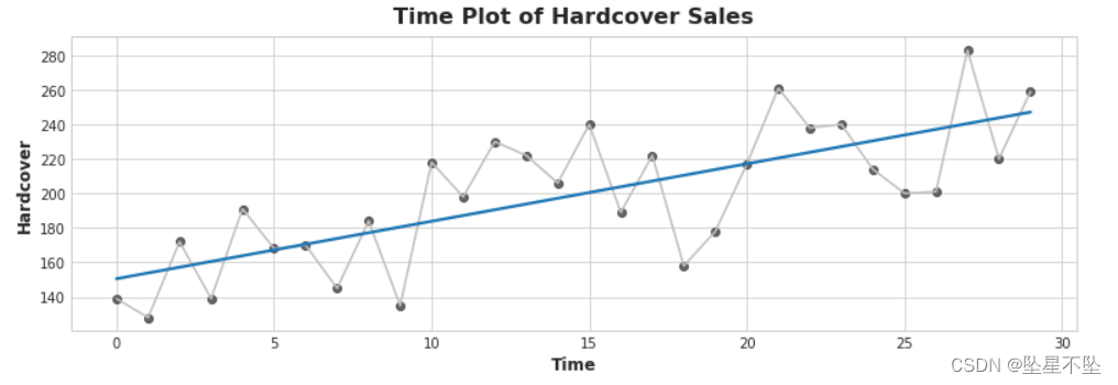

1）使用时间虚拟变量解释线性回归 

线性回归线的方程为（大约）精装书 = 3.33 * 时间 + 150.5。超过 6 天，您预计精装书销量平均会发生多大变化？在你考虑之后，运行下一个单元格

# View the solution (Run this line to receive credit!)
q_1.check()

时间变化 6 步对应于精装书销量的平均变化 6 * 3.33 = 19.98。

# Uncomment the next line for a hint
#q_1.hint()

解释回归系数可以帮助我们识别时间图中的序列依赖性。考虑模型目标 = 权重 * lag_1 + 误差，其中误差是随机噪声，权重是介于 -1 和 1 之间的数字。在这种情况下，权重告诉您下一个时间步与前一个时间步具有相同符号的可能性有多大，接近 1 的权重意味着目标可能与上一步具有相同的符号，而接近 -1 的权重意味着目标可能具有相反的符号。

2）用滞后特征解释线性回归

fig, (ax1, ax2) = plt.subplots(2, 1, figsize=(11, 5.5), sharex=True)
ax1.plot(ar['ar1'])
ax1.set_title('Series 1')
ax2.plot(ar['ar2'])
ax2.set_title('Series 2');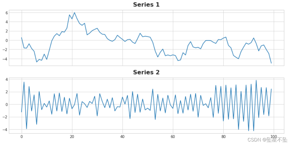

其中一个系列具有方程目标 = 0.95 * lag_1 + 误差，另一个具有方程目标 = -0.95 * lag_1 + 误差，仅在滞后特征上的符号不同。你能说出每个系列的方程式吗？

# View the solution (Run this cell to receive credit!)
q_2.check()

# Uncomment the next line for a hint
#q_2.hint()

现在我们将开始使用 Store Sales - Time Series Forecasting 竞争数据。整个数据集包含从 2013 年到 2017 年跨各种产品系列的近 1800 个系列记录商店销售额。在本课程中，我们将只处理每天平均销售额的单个系列 (average_sales)。

3) 拟合时间步长特征

完成下面的代码以创建一个线性回归模型，该模型具有一系列平均产品销售额的时间步长特征。目标位于名为“销售”的列中。

from sklearn.linear_model import LinearRegression

df = average_sales.to_frame()

# YOUR CODE HERE: Create a time dummy
time = ____

df['time'] = time 

# YOUR CODE HERE: Create training data
X = ____  # features
y = ____  # target

# Train the model
model = LinearRegression()
model.fit(X, y)

# Store the fitted values as a time series with the same time index as
# the training data
y_pred = pd.Series(model.predict(X), index=X.index)


# Check your answer
q_3.check()

# Lines below will give you a hint or solution code
#q_3.hint()
#q_3.solution()

ax = y.plot(**plot_params, alpha=0.5)
ax = y_pred.plot(ax=ax, linewidth=3)
ax.set_title('Time Plot of Total Store Sales');