前言
为了获取最佳阅读体验,建议访问个人博客:https://jmxgodlz.xyz
首先抛出关键性结论:
-
RNN模型在时间维度共享参数矩阵,因此RNN模型总的梯度等于各时间的梯度之和, g = ∑ g t g=\sum{g_t} g=∑gt。
-
RNN中总的梯度不会消失,只是远距离梯度消失,梯度被近距离梯度主导,无法捕获远距离特征。
-
梯度消失的本质:由于RNN模型在时间维度共享参数矩阵,导致针对隐藏状态h求导时,循环计算矩阵乘法,最终梯度上出现了参数矩阵的累乘。
-
LSTM缓解梯度消失的本质:引入门控机制,将矩阵乘法转为逐元素相乘的哈达马积: c t = f t ⊙ c t − 1 + i t ⊙ tanh ( W c [ h t − 1 , x t ] + b c ) c_{t}=f_{t} \odot c_{t-1}+i_{t} \odot \tanh \left(W_{c}\left[h_{t-1}, x_{t}\right]+b_{c}\right) ct=ft⊙ct−1+it⊙tanh(Wc[ht−1,xt]+bc)
梯度消失分析
基本介绍
RNN的状态更新公式如下:
h t = f ( W h t − 1 + U x t ) \begin{equation} h_t=f(Wh_{t-1}+Ux_t) \tag{1} \end{equation} ht=f(Wht−1+Uxt)(1)
y t = f ( V h t ) (2) y_t=f(Vh_t) \tag{2} yt=f(Vht)(2)
其中,h表示隐藏状态,f表示激活函数,W、U表示参数矩阵,x表示输入。从该式中可以看出不同时间维度的参数矩阵是共享的。
反向传播
我们在反向传播过程进行梯度求导,以对参数矩阵U求导为例
∂ y t ∂ U = ∂ y t ∂ h t ∂ h t ∂ U (3) \frac{\partial y_{t}}{\partial U}=\frac{\partial y_{t}}{\partial h_{t}}\frac{\partial h_{t}}{\partial U} \tag{3} ∂U∂yt=∂ht∂yt∂U∂ht(3)
其中
∂ h t ∂ U = ∑ s = 0 t ∂ h t ∂ h s ∂ h s ∂ U \begin{equation} \frac{\partial h_{t}}{\partial U}=\sum_{s=0}^{t}\frac{\partial h_{t}}{\partial h_s}\frac{\partial h_{s}}{\partial U} \tag{4} \end{equation} ∂U∂ht=s=0∑t∂hs∂ht∂U∂hs(4)
∂ h t ∂ h s = ∂ h t ∂ h t − 1 ∂ h t − 1 ∂ h t − 2 … ∂ h s + 1 ∂ h s (5) \frac{\partial h_{t}}{\partial h_{s}}=\frac{\partial h_{t}}{\partial h_{t-1}} \frac{\partial h_{t-1}}{\partial h_{t-2}} \ldots \frac{\partial h_{s+1}}{\partial h_{s}} \tag{5} ∂hs∂ht=∂ht−1∂ht∂ht−2∂ht−1…∂hs∂hs+1(5)
从式(1)(2)中可以递推到 h 0 h_0 h0,每一个隐藏状态h均与参数矩阵有关,最后的梯度 y t y_t yt依赖于每一个隐藏状态。
以 y 2 为例 , y 2 = f ( V h 2 ) = f ( V f ( W h 1 + U x 1 ) ) = f ( V f ( W f ( W h 0 + U x 0 ) + U x 1 ) ) 以y_2为例,y_2=f(Vh_2)=f(Vf(Wh_1+Ux_1))=f(Vf(Wf(Wh_0+Ux_0)+Ux_1)) 以y2为例,y2=f(Vh2)=f(Vf(Wh1+Ux1))=f(Vf(Wf(Wh0+Ux0)+Ux1)),通过全微分求导, h t h_t ht对 U , h t − 1 U,h_{t-1} U,ht−1求偏导数
∂ y 2 ∂ U = ∂ y 2 ∂ h 2 ∂ h 2 ∂ U = ∂ y 2 ∂ h 2 ( ∂ h 2 ∂ h 1 ∗ ∂ h 1 ∂ U + ∂ h 2 ∂ U ) = ∂ y 2 ∂ h 2 ( ∂ h 2 ∂ h 1 ∗ ( ∂ h 1 ∂ h 0 ∗ ∂ h 0 ∂ U + ∂ h 1 ∂ U ) + ∂ h 2 ∂ U ) = ∂ y 2 ∂ h 2 ( ∂ h 2 ∂ U + ∂ h 2 ∂ h 1 ∂ h 1 ∂ U + ∂ h 2 ∂ h 1 ∂ h 1 ∂ h 0 ∂ h 0 ∂ U ) (6) \begin{aligned} \frac{\partial y_{2}}{\partial U}&=\frac{\partial y_{2}}{\partial h_{2}} \frac{\partial h_{2}}{\partial U} \\ &= \frac{\partial y_{2}}{\partial h_{2}} (\frac{\partial h_{2}}{\partial h_{1}} * \frac{\partial h_{1}}{\partial U} + \frac{\partial h_{2}}{\partial U}) \\ &= \frac{\partial y_{2}}{\partial h_{2}} (\frac{\partial h_{2}}{\partial h_{1}} * (\frac{\partial h_{1}}{\partial h_{0}} * \frac{\partial h_{0}}{\partial U} + \frac{\partial h_{1}}{\partial U}) + \frac{\partial h_{2}}{\partial U}) \\ &=\frac{\partial y_{2}}{\partial h_{2}} (\frac{\partial h_{2}}{\partial U} + \frac{\partial h_{2}}{\partial h_1} \frac{\partial h_{1}}{\partial U} + \frac{\partial h_{2}}{\partial h_1} \frac{\partial h_{1}}{\partial h_0} \frac{\partial h_{0}}{\partial U}) \end{aligned} \tag{6} ∂U∂y2=∂h2∂y2∂U∂h2=∂h2∂y2(∂h1∂h2∗∂U∂h1+∂U∂h2)=∂h2∂y2(∂h1∂h2∗(∂h0∂h1∗∂U∂h0+∂U∂h1)+∂U∂h2)=∂h2∂y2(∂U∂h2+∂h1∂h2∂U∂h1+∂h1∂h2∂h0∂h1∂U∂h0)(6)
设 : z t = W h t − 1 + U x t (7) 设:z_t=Wh_{t-1}+Ux_t \tag{7} 设:zt=Wht−1+Uxt(7)
z t z_t zt代表未经过激活函数的神经网络输出,式(1)转化为:
h t = f ( z t ) (8) h_t=f(z_t) \tag{8} ht=f(zt)(8)
∂ h t ∂ h t − 1 = ∂ h t ∂ z t ∂ z t ∂ h t − 1 (9) \frac{\partial h_{t}}{\partial h_{t-1}}=\frac{\partial h_{t}}{\partial z_{t}} \frac{\partial z_{t}}{\partial h_{t-1}} \tag{9} ∂ht−1∂ht=∂zt∂ht∂ht−1∂zt(9)
式(8)可以拆分为两部分:
∂ z t ∂ h t − 1 = W (10) \frac{\partial z_{t}}{\partial h_{t-1}} = W \tag{10} ∂ht−1∂zt=W(10)
∂ h t ∂ z t = ( ∂ h t , 1 ∂ z t , 1 ∂ h t , 1 ∂ z t , 2 ⋯ ∂ h t , 1 ∂ z t , n ⋮ ⋮ ⋱ ⋮ ∂ h t , n ∂ z t , 1 ∂ h t , n ∂ z t , 2 ⋯ ∂ h t , n ∂ z t , n ) (11) \frac{\partial h_{t}}{\partial z_{t}}=\left(\begin{array}{cccc}\frac{\partial h_{t, 1}}{\partial z_{t, 1}} & \frac{\partial h_{t, 1}}{\partial z_{t, 2}} & \cdots & \frac{\partial h_{t, 1}}{\partial z_{t, n}} \\ \vdots & \vdots & \ddots & \vdots \\ \frac{\partial h_{t, n}}{\partial z_{t, 1}} & \frac{\partial h_{t, n}}{\partial z_{t, 2}} & \cdots & \frac{\partial h_{t, n}}{\partial z_{t, n}}\end{array}\right) \tag{11} ∂zt∂ht=⎝ ⎛∂zt,1∂ht,1⋮∂zt,1∂ht,n∂zt,2∂ht,1⋮∂zt,2∂ht,n⋯⋱⋯∂zt,n∂ht,1⋮∂zt,n∂ht,n⎠ ⎞(11)
其中, h t h_t ht元素由 z t z_t zt逐元素激活得到,因此两者对应元素才具有依赖关系,未对应元素无依赖关系,导数为0,式(10)成为一个对角矩阵.
∂ h t ∂ z t = ( f ′ ( z t , 1 ) 0 ⋯ 0 ⋮ ⋮ ⋱ ⋮ 0 0 ⋯ f ′ ( z t , n ) ) = d i a g [ f ′ ( z t ) ] (12) \frac{\partial h_{t}}{\partial z{t}}=\left(\begin{array}{cccc}f^{\prime}\left(\text { z}_{t, 1}\right) & 0 & \cdots & 0 \\ \vdots & \vdots & \ddots & \vdots \\ 0 & 0 & \cdots & f^{\prime}\left(z_{t, n}\right)\end{array}\right)=diag[f^{\prime}(z_t)] \tag{12} ∂zt∂ht=⎝ ⎛f′( zt,1)⋮00⋮0⋯⋱⋯0⋮f′(zt,n)⎠ ⎞=diag[f′(zt)](12)
根据式(9)(11),式(5)求解得到:
∂ h t ∂ h s = ∏ k = s + 1 t W T diag [ f ′ ( z k ) ] (13) \frac{\partial h_{t}}{\partial h_{s}}=\prod_{k=s+1}^{t} W^{T} \operatorname{diag}\left[f^{\prime}\left(\operatorname{z}_{k}\right)\right] \tag{13} ∂hs∂ht=k=s+1∏tWTdiag[f′(zk)](13)
在式(12)中已经出现了矩阵的连乘,根据矩阵的相容性" ∣ ∣ X Y ∣ ∣ ≤ ∣ ∣ X ∣ ∣ ∣ ∣ Y ∣ ∣ ||X Y|| \le ||X|| ||Y|| ∣∣XY∣∣≤∣∣X∣∣∣∣Y∣∣"
∣ ∣ ∂ h t ∂ h s ∣ ∣ = ∏ k = s + 1 t ∣ ∣ W T diag [ f ′ ( z k ) ] ∣ ∣ ≤ ∏ k = s + 1 t ∣ ∣ W T ∣ ∣ ∣ ∣ diag [ f ′ ( z k ) ] ∣ ∣ ≤ ∏ k = s + 1 t σ m a x γ = ( σ m a x γ ) t − s (14) \begin{aligned} ||\frac{\partial h_{t}}{\partial h_{s}}||&=\prod_{k=s+1}^{t} || W^{T} \operatorname{diag}\left[f^{\prime}\left(\operatorname{z}_{k}\right)\right]|| \\ &\le \prod_{k=s+1}^{t} ||W^{T}|| ||\operatorname{diag}\left[f^{\prime}\left(\operatorname{z}_{k}\right)\right]|| \\ &\le \prod_{k=s+1}^{t} \sigma_{max} \gamma = (\sigma_{max} \gamma)^{t-s} \end{aligned} \tag{14} ∣∣∂hs∂ht∣∣=k=s+1∏t∣∣WTdiag[f′(zk)]∣∣≤k=s+1∏t∣∣WT∣∣∣∣diag[f′(zk)]∣∣≤k=s+1∏tσmaxγ=(σmaxγ)t−s(14)
其中, σ \sigma σ 代表矩阵W的最大奇异解, γ \gamma γ代表激活函数f的上界,例如双曲正切函数的上界为 ∣ ∣ t a n h ′ ( x ) ∣ ∣ ≤ 1 ||tanh^{'}(x)|| \le 1 ∣∣tanh′(x)∣∣≤1,sigmoid函数的上界为 ∣ ∣ s i g m o i d ′ ( x ) ≤ 1 4 ∣ ∣ ||sigmoid^{'}(x) \le \frac{1}{4}|| ∣∣sigmoid′(x)≤41∣∣。
因此在远距离依赖,即t-s较大的情况下,当 σ m a x γ < 1 \sigma_{max} \gamma \lt 1 σmaxγ<1时,会发生梯度消失;当 σ m a x γ > 1 \sigma_{max} \gamma \gt 1 σmaxγ>1时,会发生梯度爆炸。
**TIPS:**这里只是不等式情况,因此即使不等式右边远大于1,也有可能发生梯度消失。但是,在实际情况下,矩阵范数的约束与实际值相当接近。
补充说明
对于传统RNN模型,在训练初期避免梯度消失与参数矩阵的初始化,即最大奇异解 σ \sigma σ值有关。
避免梯度消失的矩阵最小初始化方式如下:
以双曲正切函数为例,双曲正切函数的 γ = 1 \gamma = 1 γ=1,为了使 σ m a x γ = 1 \sigma_{max} \gamma = 1 σmaxγ=1,即 σ = 1 \sigma=1 σ=1。
为了使不等式置信度更高,将矩阵W的所有奇异解设置为1.
对于每一列而言, Σ i w i j 2 = 1 \Sigma_{i} w_{i j}^{2}=1 Σiwij2=1,其中j代表第j列,矩阵中每个元素是一个n维向量,i代表矩阵第i行,w代表列向量。
n E ( w 2 ) = 1 n \mathbb{E}\left(w^{2}\right)=1 nE(w2)=1,
我们假设w服从均匀分布,区间为 [ − R , R ] [-R,R] [−R,R],均匀分布的均值为0,方差 E ( w 2 ) = R 2 3 \mathbb{E}\left(w^{2}\right)=\frac{R^2}{3} E(w2)=3R2【均匀分布方差为 ( b − a ) 2 12 \frac{(b-a)^2}{12} 12(b−a)2】。
代入得到 n R 2 3 = 1 (15) n\frac{R^2}{3}=1 \tag{15} n3R2=1(15)
即 R = 3 n (16) R=\frac{\sqrt{3}}{\sqrt{n}} \tag{16} R=n3(16)
因此w符合的分布为 [ − 3 n , 3 n ] [-\frac{\sqrt{3}}{\sqrt{n}}, \frac{\sqrt{3}}{\sqrt{n}}] [−n3,n3],当矩阵是方阵时的Xavier-Glorot initialization分布;当矩阵行列不同时,Xavier-Glorot initialization分布为 [ − 6 m + n , 6 m + n ] \left[-\frac{\sqrt{6}}{\sqrt{m+n}}, \frac{\sqrt{6}}{\sqrt{m+n}}\right] [−m+n6,m+n6]。
LSTM提出
关于RNN反向传播的一些评论:
- RNN模型在时间维度共享参数矩阵
- 权重更新的频率与梯度的准确性需要权衡,越少的更新次数,梯度准确性越高,但训练速度也下降了。【由反向传递时,使用上一时刻状态做近似导致】
- 梯度消失带来不稳定的梯度流;共享参数带来对最新更新的过度敏感
- 针对上述三点,进行错误传播过程的梯度截断是有必要的
- 传播梯度分量也是可以的
LSTM缓解梯度消失的根本方法:write it down【将状态记录下来】,但是如果无限制的写入也会带来问题,因此升级为有选择的读写,这样带来了LSTM的三个关键机制:
- 有选择的写入,写入关键信息
- 有选择的读取信息
- 有选择的遗忘信息
我们可以通过门机制实现选择性,但要如何将这三个机制结合起来呢?
LSTM原型
首先,提出一个LSTM原型,本着先读取状态,再写入的原则,每一次更新状态的增量 s ~ t \tilde{s}_{t} s~t,由 o t o_t ot选择性读取上一个状态的内容, i t i_t it为选择写入, f t f_t ft选择性遗忘上一状态的内容:
i t = σ ( W i s t − 1 + U i x t + b i ) o t = σ ( W o s t − 1 + U o x t + b o ) f t = σ ( W f s t − 1 + U f x t + b f ) s t ~ = ϕ ( W ( o t ⊙ s t − 1 ) + U x t + b ) s t = f t ⊙ s t − 1 + i t ⊙ s ~ t (17) \begin{aligned} i_{t} &=\sigma\left(W_{i} s_{t-1}+U_{i} x_{t}+b_{i}\right) \\ o_{t} &=\sigma\left(W_{o} s_{t-1}+U_{o} x_{t}+b_{o}\right) \\ f_{t} &=\sigma\left(W_{f} s_{t-1}+U_{f} x_{t}+b_{f}\right) \\ \tilde{s_{t}} &=\phi\left(W\left(o_{t} \odot s_{t-1}\right)+U x_{t}+b\right) \\ s_{t} &=f_{t} \odot s_{t-1}+i_{t} \odot \tilde{s}_{t} \end{aligned} \tag{17} itotftst~st=σ(Wist−1+Uixt+bi)=σ(Wost−1+Uoxt+bo)=σ(Wfst−1+Ufxt+bf)=ϕ(W(ot⊙st−1)+Uxt+b)=ft⊙st−1+it⊙s~t(17)

三个起效果的改进版本
按理说上述LSTM原型能够起效果,但事与愿违,**选择性读取与选择性写入未能很好的协调,导致状态值非常大,紧接着门机制变得饱和。**这种情况源于的 s t s_t st是无界的,会变得非常大从而导致门机制饱和,因此接下来的三个改进的生效版本均是约束 s t s_t st的大小,将其约束成有界。
归一化LSTM原型
针对 s t s_t st进行正态归一化, s t = s t − m e a n ( s t ) V a r ( s t ) + 1 s_t = \frac{s_t-mean(s_t)}{\sqrt{Var(s_t) + 1}} st=Var(st)+1st−mean(st),也可以类似于层归一化等方式添加缩放与平移分量。
归一化后的 s t s_t st从无界成为有界。
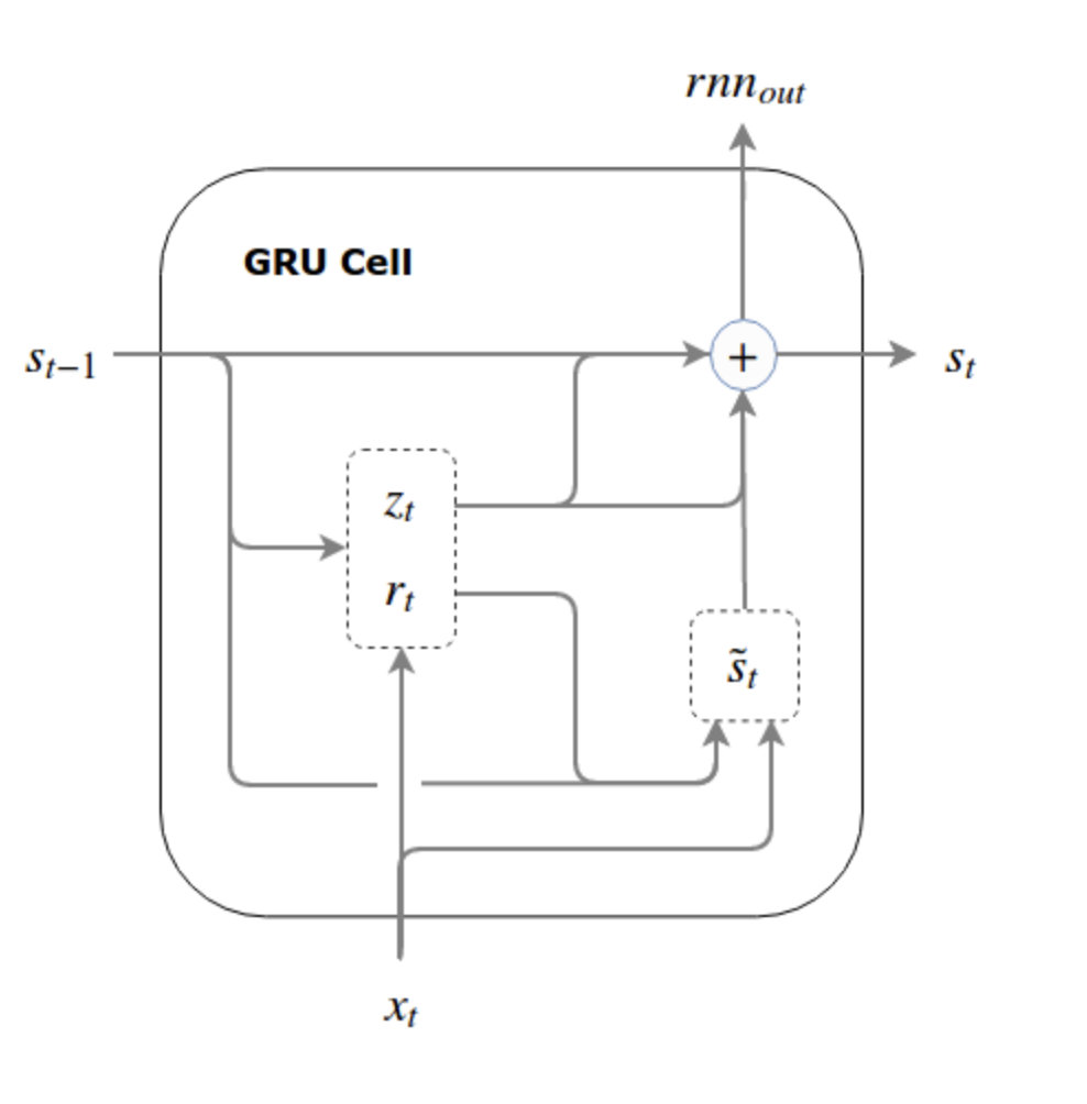
GRU:将写入与遗忘强绑定
s t = ( 1 − i t ) ⊙ s t − 1 + i t ⊙ s ~ t (18) s_{t}=\left(1-i_{t}\right) \odot s_{t-1}+i_{t} \odot \tilde{s}_{t} \tag{18} st=(1−it)⊙st−1+it⊙s~t(18)
GRU将写入门与遗忘门绑定起来,使之加和为1。将 s t s_t st变成 s t − 1 s_{t-1} st−1与 s ~ t \tilde{s}_{t} s~t的element-wise加权平均,当两者均有界时, s t s_t st也有界。
以下给出GRU的计算公式,与原理图:
r t = σ ( W r s t − 1 + U r x t + b r ) z t = σ ( W z s t − 1 + U z x t + b z ) s t ~ = ϕ ( W ( r t ⊙ s t − 1 ) + U x t + b ) s t = z t ⊙ s t − 1 + ( 1 − z t ) ⊙ s ~ t (19) \begin{aligned} r_{t} &=\sigma\left(W_{r} s_{t-1}+U_{r} x_{t}+b_{r}\right) \\ z_{t} &=\sigma\left(W_{z} s_{t-1}+U_{z} x_{t}+b_{z}\right) \\ \tilde{s_{t}} &=\phi\left(W\left(r_{t} \odot s_{t-1}\right)+U x_{t}+b\right) \\ s_{t} &=z_{t} \odot s_{t-1}+\left(1-z_{t}\right) \odot \tilde{s}_{t} \end{aligned} \tag{19} rtztst~st=σ(Wrst−1+Urxt+br)=σ(Wzst−1+Uzxt+bz)=ϕ(W(rt⊙st−1)+Uxt+b)=zt⊙st−1+(1−zt)⊙s~t(19)
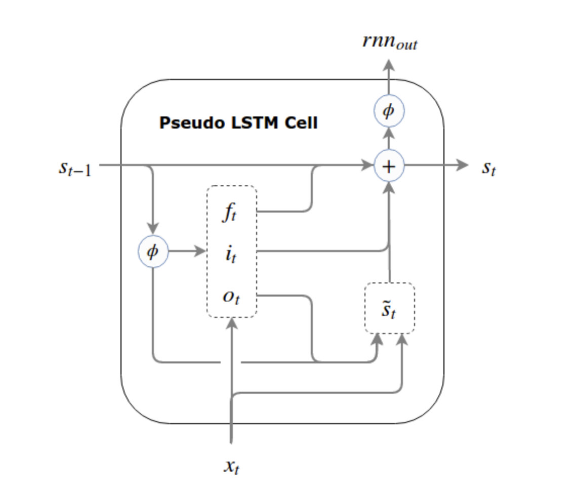
伪LSTM:通过激活函数约束
通过激活函数,将 s t s_t st限制到激活函数的上界内。
只有在更新写入时,为了避免信息的变化,未使用激活函数约束。
以下给出伪LSTM的计算公式,与原理图:
i t = σ ( W i ( ϕ ( s t − 1 ) ) + U i x t + b i ) o t = σ ( W o ( ϕ ( s t − 1 ) ) + U o x t + b o ) f t = σ ( W f ( ϕ ( s t − 1 ) ) + U f x t + b f ) s ~ t = ϕ ( W ( o t ⊙ ϕ ( s t − 1 ) ) + U x t + b ) s t = f t ⊙ s t − 1 + i t ⊙ s ~ t r n n out = ϕ ( s t ) (20) \begin{aligned} i_{t} &=\sigma\left(W_{i}\left(\phi\left(s_{t-1}\right)\right)+U_{i} x_{t}+b_{i}\right) \\ o_{t} &=\sigma\left(W_{o}\left(\phi\left(s_{t-1}\right)\right)+U_{o} x_{t}+b_{o}\right) \\ f_{t} &=\sigma\left(W_{f}\left(\phi\left(s_{t-1}\right)\right)+U_{f} x_{t}+b_{f}\right) \\ \tilde{s}_{t} &=\phi\left(W\left(o_{t} \odot \phi\left(s_{t-1}\right)\right)+U x_{t}+b\right) \\ s_{t} &=f_{t} \odot s_{t-1}+i_{t} \odot \tilde{s}_{t} \\ \mathbf{r n n}_{\text {out }} &=\phi\left(s_{t}\right) \end{aligned} \tag{20} itotfts~tstrnnout =σ(Wi(ϕ(st−1))+Uixt+bi)=σ(Wo(ϕ(st−1))+Uoxt+bo)=σ(Wf(ϕ(st−1))+Ufxt+bf)=ϕ(W(ot⊙ϕ(st−1))+Uxt+b)=ft⊙st−1+it⊙s~t=ϕ(st)(20)
LSTM提出
LSTM与伪LSTM的几点关键区别如下:
-
LSTM是先写后读,因此添加了一个“影子”状态,Hochreiter and Schmidhuber等人认为状态s与剩余的RNN cell是独立的。
-
使用门控影子状态 h t − 1 = o t − 1 ⊙ ϕ ( c t − 1 ) h_{t-1}=o_{t-1}\odot \phi(c_{t-1}) ht−1=ot−1⊙ϕ(ct−1)计算门结构,替换激活后的 ϕ ( c t − 1 ) \phi(c_{t-1}) ϕ(ct−1)。这样隐藏状态均是当前时间下的信息,与读取信息时 ( o t ⊙ s t − 1 ) (o_t \odot s_{t-1}) (ot⊙st−1)利用前一时刻信息不同。
-
使用门控影子状态作为RNN cell的输出 h t = o t ⊙ ϕ ( c t ) h_{t}=o_{t}\odot \phi(c_{t}) ht=ot⊙ϕ(ct),替代 ϕ ( c t ) \phi(c_t) ϕ(ct)。
这样一来,LSTM的输入就是上一时刻的 c t − 1 , h t − 1 c_{t-1},h_{t-1} ct−1,ht−1,输出为 c t , h t c_t,h_t ct,ht。
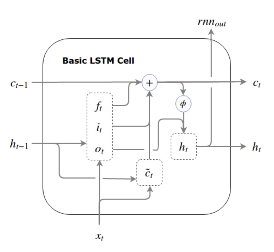
基础LSTM
基础LSTM单元的公式与原理图如下:
i t = σ ( W i h t − 1 + U i x t + b i ) o t = σ ( W o h t − 1 + U o x t + b o ) f t = σ ( W f h t − 1 + U f x t + b f ) c ~ t = ϕ ( W h t − 1 + U x t + b ) c t = f t ⊙ c t − 1 + i t ⊙ c ~ t h t = o t ⊙ ϕ ( c t ) r n n out = h t (21) \begin{aligned} i_{t} &=\sigma\left(W_{i} h_{t-1}+U_{i} x_{t}+b_{i}\right) \\ o_{t} &=\sigma\left(W_{o} h_{t-1}+U_{o} x_{t}+b_{o}\right) \\ f_{t} &=\sigma\left(W_{f} h_{t-1}+U_{f} x_{t}+b_{f}\right) \\ \tilde{c}_{t} &=\phi\left(W h_{t-1}+U x_{t}+b\right) \\ c_{t} &=f_{t} \odot c_{t-1}+i_{t} \odot \tilde{c}_{t} \\ h_{t} &=o_{t} \odot \phi\left(c_{t}\right) \\ \mathrm{rnn}_{\text {out }} &=h_{t} \end{aligned} \tag{21} itotftc~tcthtrnnout =σ(Wiht−1+Uixt+bi)=σ(Woht−1+Uoxt+bo)=σ(Wfht−1+Ufxt+bf)=ϕ(Wht−1+Uxt+b)=ft⊙ct−1+it⊙c~t=ot⊙ϕ(ct)=ht(21)
The LSTM with peepholes
利用前一状态 c t − 1 c_{t-1} ct−1来进行门控机制的计算,但输出利用实时信息 c t c_t ct。
计算公式如下:
i t = σ ( W i h t − 1 + U i x t + P i c t − 1 + b i ) f t = σ ( W f h t − 1 + U f x t + P f c t − 1 + b f ) c ~ t = ϕ ( W h t − 1 + U x t + b ) c t = f t ⊙ c t − 1 + i t ⊙ c ~ t o t = σ ( W o h t − 1 + U o x t + P o c t + b o ) h t = o t ⊙ ϕ ( c t ) rnn out = h t (22) \begin{aligned} i_{t} &=\sigma\left(W_{i} h_{t-1}+U_{i} x_{t}+P_{i} c_{t-1}+b_{i}\right) \\ f_{t} &=\sigma\left(W_{f} h_{t-1}+U_{f} x_{t}+P_{f} c_{t-1}+b_{f}\right) \\ \tilde{c}_{t} &=\phi\left(W h_{t-1}+U x_{t}+b\right) \\ c_{t} &=f_{t} \odot c_{t-1}+i_{t} \odot \tilde{c}_{t} \\ o_{t} &=\sigma\left(W_{o} h_{t-1}+U_{o} x_{t}+P_{o} c_{t}+b_{o}\right) \\ h_{t} &=o_{t} \odot \phi\left(c_{t}\right) \\ \operatorname{rnn}_{\text {out }} &=h_{t} \end{aligned} \tag{22} itftc~tctothtrnnout =σ(Wiht−1+Uixt+Pict−1+bi)=σ(Wfht−1+Ufxt+Pfct−1+bf)=ϕ(Wht−1+Uxt+b)=ft⊙ct−1+it⊙c~t=σ(Woht−1+Uoxt+Poct+bo)=ot⊙ϕ(ct)=ht(22)
LSTM如何解决梯度消失
从上述分析可以得到,梯度消失中最大原因是需要计算 ∂ h t ∂ h s \frac{\partial h_{t}}{\partial h_{s}} ∂hs∂ht,如果这个值不随着层数的增加,趋于0或者无穷大,那么就能够捕获到长距离依赖信息。
LSTM将状态与其他部分分开,状态更新部分变成:
c t = f t ⊙ c t − 1 + i t ∗ c ~ t = c t = f t ⊙ c t − 1 + i t ⊙ tanh ( W c [ h t − 1 , x t ] + b c ) (23) c_t = f_t \odot c_{t-1} + i_t * \tilde c_t = c_{t}=f_{t} \odot c_{t-1}+i_{t} \odot \tanh \left(W_{c}\left[h_{t-1}, x_{t}\right]+b_{c}\right) \tag{23} ct=ft⊙ct−1+it∗c~t=ct=ft⊙ct−1+it⊙tanh(Wc[ht−1,xt]+bc)(23)
针对状态进行求导,同时 c t c_t ct与 c t − 1 , c ~ t − 1 , f t , i t c_{t-1},\tilde c_{t-1},f_t,i_t ct−1,c~t−1,ft,it有关,因此进行全微分求导
∂ C t ∂ C t − 1 = ∂ C t ∂ C t − 1 + ∂ C t ∂ C ~ t ∗ ∂ C ~ t ∂ C t − 1 + ∂ C t ∂ i t ∗ ∂ i t ∂ C t − 1 + ∂ C t ∂ f t ∗ ∂ f t ∂ C t − 1 = ∂ C t ∂ C t − 1 + ∂ C t ∂ C ~ t ∗ ∂ C ~ t ∂ h t − 1 ∗ ∂ h t − 1 ∂ C t − 1 + ∂ C t ∂ i t ∗ ∂ i t ∂ h t − 1 ∗ ∂ h t − 1 ∂ C t − 1 + ∂ C t ∂ f t ∗ ∂ f t ∂ h t − 1 ∗ ∂ h t − 1 ∂ C t − 1 = f t + i t ∗ t a n h ′ ( ∗ ) W c ∗ o t − 1 t a n h ′ ( C t − 1 ) + C ~ t ∗ σ ′ ( ∗ ) W i ∗ o t − 1 t a n h ′ ( C t − 1 ) + C t − 1 ∗ σ ′ ( ∗ ) W f ∗ o t − 1 t a n h ′ ( C t − 1 ) (24) \begin{aligned} \frac{\partial C_{t}}{\partial C_{t-1}} &= \frac{\partial C_{t}}{\partial C_{t-1}} + \frac{\partial C_{t}}{\partial \tilde C_{t}} * \frac{\partial \tilde C_{t}}{\partial C_{t-1}} + \frac{\partial C_{t}}{\partial i_{t}} * \frac{\partial i_{t}}{\partial C_{t-1}} + \frac{\partial C_{t}}{\partial f_{t}} * \frac{\partial f_{t}}{\partial C_{t-1}} \\ &=\frac{\partial C_{t}}{\partial C_{t-1}} + \frac{\partial C_{t}}{\partial \tilde C_{t}} * \frac{\partial \tilde C_{t}}{\partial h_{t-1}} * \frac{\partial h_{t-1}}{\partial C_{t-1}} \\ &+ \frac{\partial C_{t}}{\partial i_{t}} * \frac{\partial i_{t}}{\partial h_{t-1}} * \frac{\partial h_{t-1}}{\partial C_{t-1}} + \frac{\partial C_{t}}{\partial f_{t}} * \frac{\partial f_{t}}{\partial h_{t-1}} * \frac{\partial h_{t-1}}{\partial C_{t-1}} \\ &= f_t + i_t * tanh^{'}(*)W_c * o_{t-1} tanh^{'}(C_{t-1}) \\ &+ \tilde C_t * \sigma^{'}(*)W_i * o_{t-1} tanh^{'}(C_{t-1}) + C_{t-1} * \sigma^{'}(*)W_f * o_{t-1} tanh^{'}(C_{t-1}) \end{aligned} \tag{24} ∂Ct−1∂Ct=∂Ct−1∂Ct+∂C~t∂Ct∗∂Ct−1∂C~t+∂it∂Ct∗∂Ct−1∂it+∂ft∂Ct∗∂Ct−1∂ft=∂Ct−1∂Ct+∂C~t∂Ct∗∂ht−1∂C~t∗∂Ct−1∂ht−1+∂it∂Ct∗∂ht−1∂it∗∂Ct−1∂ht−1+∂ft∂Ct∗∂ht−1∂ft∗∂Ct−1∂ht−1=ft+it∗tanh′(∗)Wc∗ot−1tanh′(Ct−1)+C~t∗σ′(∗)Wi∗ot−1tanh′(Ct−1)+Ct−1∗σ′(∗)Wf∗ot−1tanh′(Ct−1)(24)
从上式可以得到, ∂ C t ∂ C t − 1 \frac{\partial C_{t}}{\partial C_{t-1}} ∂Ct−1∂Ct成为上述4部分的加和,在连乘的任意时刻可能是 [ 0 , + ∞ ) [0, +\infty) [0,+∞)的范围,并不会一直趋于0,或者 ∞ \infty ∞。同时 f t , i t , o t − 1 , C ~ t f_t,i_t,o_{t-1},\tilde C_t ft,it,ot−1,C~t都是网络学习的值,也就是说由网络自己学习哪些梯度保留,哪些梯度剔除。
在这些机制的帮助下,LSTM很好的缓解了梯度消失问题。
LSTM延伸
Highway网络和residual网络同样包含了LSTM最基本的思想:与原先一层网络输出 x t + 1 = N e t ( x t ) x_{t + 1} = Net(x_t) xt+1=Net(xt)的计算方式相比,计算增量 x t + 1 = x t + Δ x t + 1 x_{t + 1} = x_t + \Delta x_{t + 1} xt+1=xt+Δxt+1。
因此这两种方式,同样会遇到LSTM的问题:读写的不协调。
关于这两者的介绍,再后续有时间展开进行介绍。
参考文献
https://www.zhihu.com/question/34878706
https://r2rt.com/written-memories-understanding-deriving-and-extending-the-lstm.html
https://www.zhihu.com/question/34878706
https://zhuanlan.zhihu.com/p/109519044
https://weberna.github.io/blog/2017/11/15/LSTM-Vanishing-Gradients.html?utm_source=wechat_session&utm_medium=social&utm_oi=1088177386838749184