记录 CLIP 论文阅读、zero-shot实验（直接推理）、linear probe实验（冻结CLIP抽特征只训练分类层）。

一、论文阅读

Paper：Learning Transferable Visual Models From Natural Language Supervision
Github：https://github.com/openai/CLIP
参考视频：CLIP 论文逐段精读【论文精读】

CLIP（Contrastive Language-Image Pre-training）是 2021 年 OpenAI 的一篇工作，目的是用文本作为监督信号训练可迁移的视觉模型，模型原理如下红框所示：

在这里插入图片描述

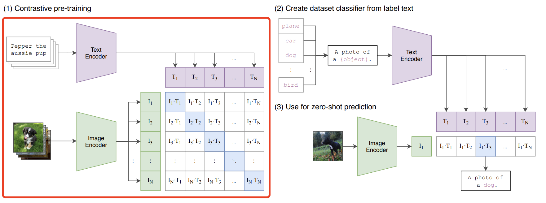
Text Encoder：用的是 Transformer，12层，8个head，512维特征，分词器用 BPE 字节对编码；
Image Encoder：实验时选了5个不同的 ResNet、EfficientNet 和 3 个不同的 ViT，最终选用 ViT-L/14@336px。

具体模型超参如下：
在这里插入图片描述

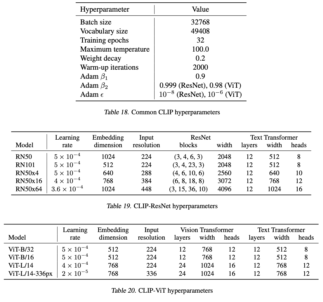
训练阶段：预训练目标通过对比学习，让模型学习文本-图像对的匹配关系，也就是上面模型原理图中，蓝色对角线为匹配的图文对。训练集用的他们自己采集的包含4亿个图文对的 WIT（WebImageText）数据集。
推理阶段：用 prompt engineering（比如图像狗猫二分类，分别输入 “ A photo of cat ” 和 “ A photo of dog ”，然后分别跟图像特征算相似度）和 prompt ensemble（设计了80多个prompt，比如可以对 “cat”、“dog” 用不同的prompt构造输入文本，分别抽特征然后打分）。

以下是模型工作流程的伪代码：

# image_encoder - 残差网络 ResNet 或者 Vision Transformer
# text_encoder - CBOW 或者文本 Transformer

# I[n, h, w, c] - 训练图像，n是batch size，h/w/c分别是高/宽/通道数
# T[n, l] - 训练文本，n是batch size，l是文本长度
# W_i[d_i, d_e] - 可学习的 图像嵌入 投影矩阵
# W_t[d_t, d_e] - 可学习的 文本嵌入 投影矩阵
# t - softmax 可学习的 temperature 参数

# 抽特征 I_f 和 T_f
I_f = image_encoder(I) #[n, d_i]
T_f = text_encoder(T) #[n, d_t]

# 对 I_f、T_f 分别点乘各自投影矩阵，投到同一个向量空间，并做 norm 得到各自特征向量。[n, d_e]
I_e = l2_normalize(np.dot(I_f, W_i), axis=1)
T_e = l2_normalize(np.dot(T_f, W_t), axis=1)

# 算图文特征的余弦相似度。[n, n]
logits = np.dot(I_e, T_e.T) * np.exp(t)

# 对称损失函数（对比学习常用）
labels = np.arange(n)
loss_i = cross_entropy_loss(logits, labels, axis=0)
loss_t = cross_entropy_loss(logits, labels, axis=1)
loss = (loss_i + loss_t)/2

二、zero-shot 推理实验

本部分直接加载预训练好的模型权重进行 zero-shot 推理。

新建项目 openai_clip，参考 Github，源码安装 clip 等依赖：
```
pip install git+https://github.com/openai/CLIP.git
```

将模型权重手动下载到本地（ViT-B/32）：

wget https://openaipublic.azureedge.net/clip/models/40d365715913c9da98579312b702a82c18be219cc2a73407c4526f58eba950af/ViT-B-32.pt

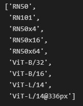
存入测试图片 piano_dog.png ，新建 zero-shot.ipynb，运行代码：

import torch
import clip
import os
import numpy as np
from PIL import Image

os.environ['CUDA_VISIBLE_DEVICES']='1'
device = "cuda" if torch.cuda.is_available() else "cpu"
clip.available_models()

测试图片：
在这里插入图片描述
可用模型权重列表：

加载模型，查看模型信息：

model, preprocess = clip.load("ckpt/ViT-B-32.pt", device=device)

input_resolution = model.visual.input_resolution
context_length = model.context_length
vocab_size = model.vocab_size

print("Model parameters:", f"{
        
        np.sum([int(np.prod(p.shape)) for p in model.parameters()]):,}")
print("Input resolution:", input_resolution)
print("Context length:", context_length)
print("Vocab size:", vocab_size)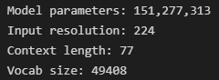

在这里插入图片描述

提取图文特征，计算相似度：

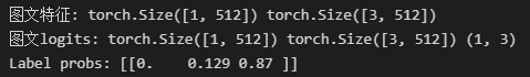
image = preprocess(Image.open("./dataset/piano_dog.png")).unsqueeze(0).to(device)
text = clip.tokenize(["a dog eating an egg", "a dog singing a song", "a dog playing a piano"]).to(device)

with torch.no_grad():

    image_features = model.encode_image(image)
    text_features = model.encode_text(text)
    print("图文特征:", image_features.shape, text_features.shape)

    logits_per_image, logits_per_text = model(image, text)
    probs = logits_per_image.softmax(dim=-1).cpu().numpy()
    print("图文logits:", image_features.shape, text_features.shape, probs.shape)

print("Label probs:", np.around(probs, 3))  # prints: [[0.9927937  0.00421068 0.00299572]]

可见，“a dog playing a piano” 的概率最大。
在这里插入图片描述

三、Linear Probe 训练实验

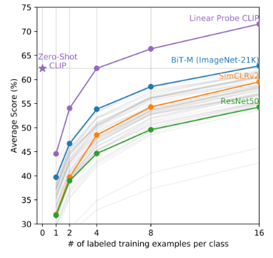
论文里提到，冻住 CLIP用来抽特征，然后加个线性层用于分类，用 8-shot 及以上的样本训一波之后，效果会比直接 zeroshot 好。所以用 sklearn 实战一下。
在这里插入图片描述

import os
import clip
import torch

import numpy as np
from sklearn.linear_model import LogisticRegression
from torch.utils.data import DataLoader
from torchvision.datasets import CIFAR100
from tqdm import tqdm

# 加载模型
device = "cuda:4" if torch.cuda.is_available() else "cpu"
model, preprocess = clip.load('./ckpt/ViT-B-32.pt', device)

# 加载 cifar100 数据集 (root 路径下需包含解压后的 cifar-100-python 文件夹)
root = os.path.expanduser("./dataset/cifar100/")
train = CIFAR100(root, download=True, train=True, transform=preprocess)
test = CIFAR100(root, download=True, train=False, transform=preprocess)

# 模型只用于提取特征
def get_features(dataset):
    all_features = []
    all_labels = []
    
    with torch.no_grad():
        for images, labels in tqdm(DataLoader(dataset, batch_size=100)):
            features = model.encode_image(images.to(device))

            all_features.append(features)
            all_labels.append(labels)

    return torch.cat(all_features).cpu().numpy(), torch.cat(all_labels).cpu().numpy()

# 构造 sklearn 的 train_X, train_y, test_X, test_y
train_features, train_labels = get_features(train)
test_features, test_labels = get_features(test)

# 初始化一个 logistic regression 对象
classifier = LogisticRegression(random_state=0, C=0.316, max_iter=1000, verbose=1)
classifier.fit(train_features, train_labels)

# 评测一下
predictions = classifier.predict(test_features)
accuracy = np.mean((test_labels == predictions).astype(np.float)) * 100.
print(f"Accuracy = {
      
      accuracy:.3f}")

CLIP论文阅读、zero-shot实验、linear prob实验记录

一、论文阅读

二、zero-shot 推理实验

三、Linear Probe 训练实验

猜你喜欢