Visual Transformer (ViT)模型与代码实现（PyTorch）

摘要

This chapter is about the pioneering application of Transformer in the CV field - the VIT model, the understanding of the VIT model and the concise code implementation process. The most critical problem solved by the VIT model is to patch the image into multiple ordered time series data, add CLS tokens, and then combine traditional post embedding to construct sequence data suitable for input into the Transformer model. The VIT model only applies the Encoder part of the Transformer model, and makes some fine-tuning of the encoder part, such as advancing the Norm operation before the attention, the generation of QKV in the attention and the division of the head are different from the traditional ones. made simpler and easier to understand. However, in order to achieve good results, the VIT model must rely on pre-training on massive datasets.

本章是对开启Transformer应用在CV领域的开山之作—VIT模型的理解与简洁代码实现过程，VIT模型解决的最关键的问题在于将图像patch成多个有序的时序数据，加入CLS token ,再结合传统的postion embedding ,构建适合输入Transformer模型的序列数据。VIT模型仅仅只是应用了Transformer 模型的Encoder部分，并对encoder部分进行一定的微调，比如将Norm操作提前在attention之前，而attention 中的QKV的生成与head 的分成，都与传统的不同，总体上变得更加简单而易懂。但是VIT模型如果想取得好的效果，必须依靠海量数据集上预训练。

上一节从NLP领域，词句如何转化成word embedding,以及怎样做postion embedding, padding mask是由NLP这类特定任务带来的,所以必须做的 encoder输入前自身 self-attention mask，与intra_attention 的mask，以及decoder 中的因果mask。 从最基础的代码实现了上述的这几个过程。具体可参考：细致理解Transforemr模型Encoder原理讲解与其Pytorch逐行实现

一. Visual Transformer (ViT)模型

论文源地址：https://arxiv.org/abs/2010.11929
参考博客地址：VIT详细讲解

1.1 ViT模型整体结构

ViT模型是基于Transformer的模型在CV视觉领域的开篇之作，本篇将尽可能简洁地介绍一下ViT模型的整体架构以及基本原理。ViT模型是基于Transformer Encoder模型的，但其实最关键的是如何将图片像素转化成时序数据，输入到Transformer模型中去，同时又要避免复杂度过大，计算量，维度过大的问题。

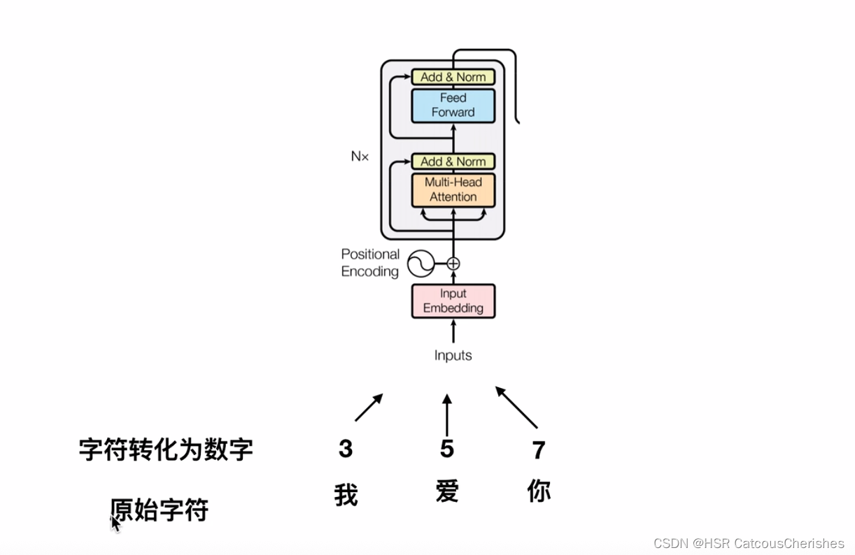
由于在NLP领域，是通过将词句字符转化成索引数字，然后再通过词表进行embedding 词向量化，过程如下图所示，其次再引入位置编码;先构成序列建模的word Embedding +postion Embedding ，作为TRM——encoder 模型输入。

怎么把图片转化成token？ , 最早方法是将每一个像素点，转化成token，将其对应的数字转换成向量；再与对应的位置编码相加。但会造成复杂度过大，最大程度将变成BERT模型512的将近100倍还要多，参数量将会暴增，复杂度将会平方级的增加！

一般的改进方法：

1. 局部注意力机制
2. 改进attention公式机制原理
3. 稀疏注意力/哈希注意力等

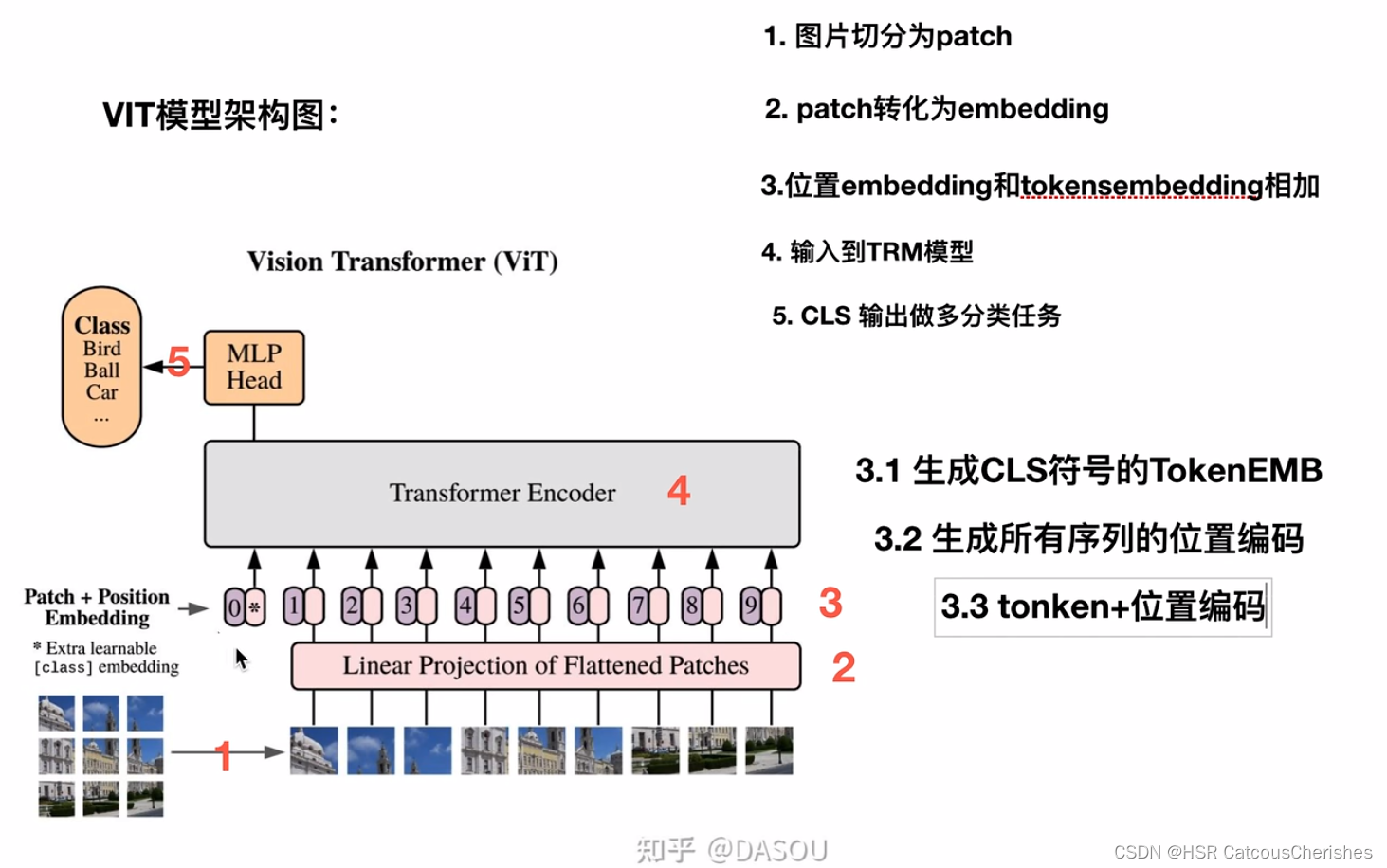
然而，VIT会是一个简单的改进方法，其将图像化整为0，切分成patch,就是一个一个的块状图像。VIT模型结构如下：

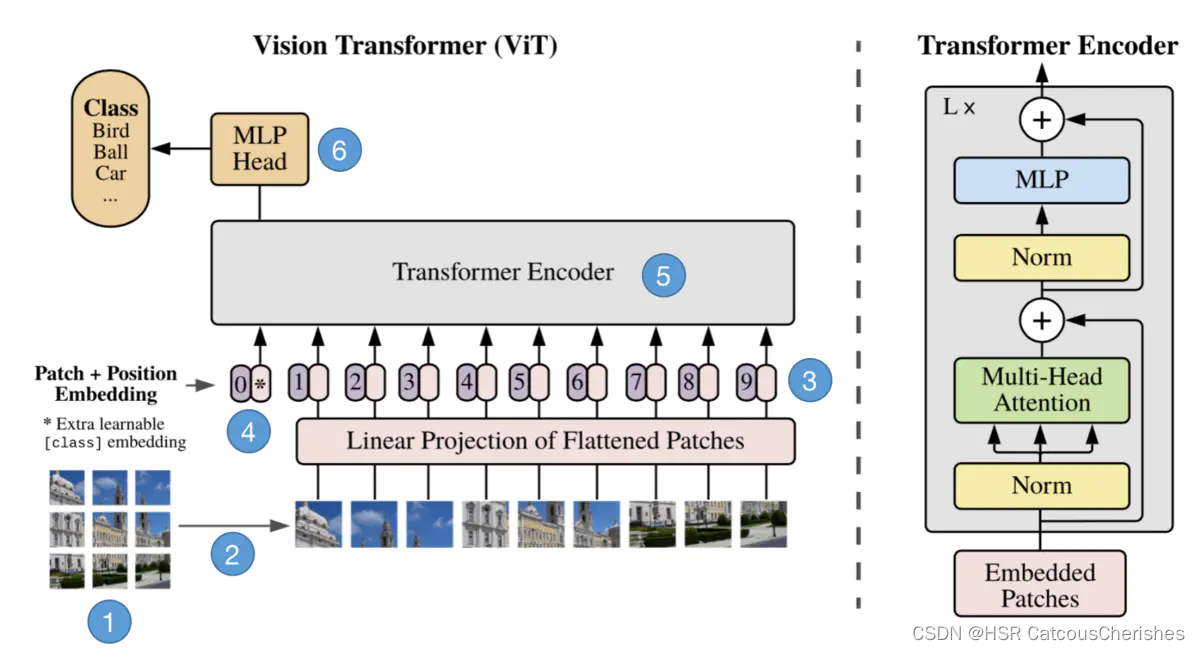
输入图片被划分为一个个16x16的小块，也叫做patch。接着这些patch被送入一个全连接层得到embeddings，然后在embeddings前再加上一个特殊的cls token。然后给所有的embedding加上位置信息编码positional encoding。接着这个整体被送入Transformer Encoder，然后取cls token的输出特征送入MLP Head去做分类，总体流程就是这样。

VIT模型上图展示的过程近一步分解为6步：

步骤１：将图片转换成patches序列

为了让Transformer能够处理图像数据，第一步必须先将图像数据转换成序列数据。假如我们有一张图片$X\in R^{H\ast W\ast C}$，patch大小为ｐ，那么我们可以创建Ｎ个图像patches，可以表示为$X_p$，其中$N=(H\ast W)/p^2$，N就是序列的长度，类似一个句子中单词的个数。

步骤2:将Patches铺平
在原论文中，作者选用的patch大小为16，那么一个patch的shape为(3,16,16)，维度为3，将它铺平之后大小为3x16x16=768。即一个patch变为长度为768的向量。不过这看起来还是有点大，此时可以使用加一个Linear transformation，即添加一个线性映射层，将patch的维度映射到我们指定的embedding的维度，这样就和NLP中的词向量类似了。

步骤3:添加Position embedding

与CNNs不同，此时模型并不知道序列数据中的patches的位置信息。所以这些patches必须先追加一个位置信息，也就是图中的带数字的向量。实验表明，不同的位置编码embedding对最终的结果影响不大，在Transformer原论文中使用的是固定位置编码，在ViT中使用的可学习的位置embedding 向量，将它们加到对应的输出patch embeddings上。

步骤4：添加class token
在输入到Transformer Encoder之前，还需要添加一个特殊的class token，这一点主要是借鉴了BERT模型。添加这个class token的目的是因为，ViT模型将这个class token在Transformer Encoder的输出当做是模型对输入图片的编码特征，用于后续输入MLP模块中与图片label进行loss计算。（其实也可以不用添加cls）

步骤5:输入Transformer Encoder
将patch embedding和class token拼接起来输入标准的Transformer Encoder中。

步骤6：多分类
注意Transformer Encoder的输出其实也是一个序列，但是在ViT模型中只使用了class token的输出，将其送入MLP模块中，去输出最终的分类结果。

1.2小结

ViT的整体思想比较简单，主要是将图片分类问题转换成了序列问题。即将图片patch转换成token，以便使用Transformer来处理。听起来很简单，但是ViT需要在海量数据集上预训练，然后在下游数据集上进行微调才能取得较好的效果，否则效果不如ResNet50等基于CNN的模型。

二. VIT 代码实现PyTorch版本

2.1 整体对比

先对比与原始Transformer论文encoder模型的不同之处：

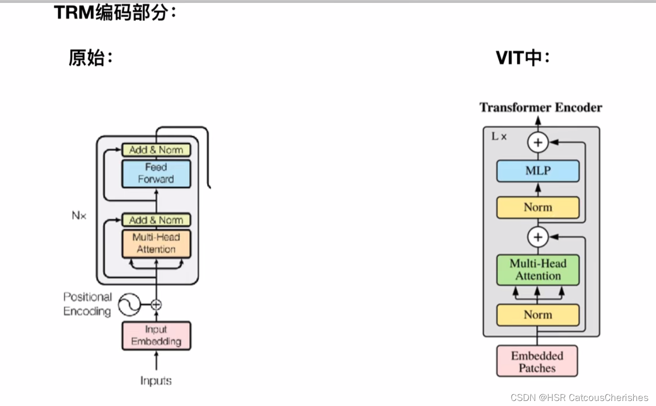
发现有着许多的不同，比如把Norm提前了，还有没有了padding (图像不存在补0的操作）。

据说Norm的位置放在前面效果会更好，所以往后的模型中Norm 大多数都是将其先进行Norm了。

2.2 整体框架代码

这里是简单一个功能模型框架

# 1. VIＴ整体架构从这里开始
class ViT(nn.Module):
    def __init__(self, *, image_size, patch_size, num_classes, dim, depth, heads, mlp_dim, pool = 'cls', channels = 3, dim_head = 64, dropout = 0., emb_dropout = 0.):
        super().__init__()
        # 初始化函数内，是将输入的图片，得到 img_size ，patch_size 的宽和高
        image_height, image_width = pair(image_size) ## 224*224 *3
        patch_height, patch_width = pair(patch_size)## 16 * 16  *3
        #图像尺寸必须能被patch大小整除
        assert image_height % patch_height == 0 and image_width % patch_width == 0, 'Image dimensions must be divisible by the patch size.'

        num_patches = (image_height // patch_height) * (image_width // patch_width) ## 步骤1.一个图像 分成 N 个patch
        patch_dim = channels * patch_height * patch_width
        assert pool in {
    
    'cls', 'mean'}, 'pool type must be either cls (cls token) or mean (mean pooling)'

        self.to_patch_embedding = nn.Sequential(
            Rearrange('b c (h p1) (w p2) -> b (h w) (p1 p2 c)', p1 = patch_height, p2 = patch_width),# 步骤2.1将patch 铺开
            nn.Linear(patch_dim, dim), # 步骤2.2 然后映射到指定的embedding的维度
        )

        self.pos_embedding = nn.Parameter(torch.randn(1, num_patches + 1, dim))
        self.cls_token = nn.Parameter(torch.randn(1, 1, dim))
        self.dropout = nn.Dropout(emb_dropout)

        self.transformer = Transformer(dim, depth, heads, dim_head, mlp_dim, dropout)

        self.pool = pool
        self.to_latent = nn.Identity()

        self.mlp_head = nn.Sequential(
            nn.LayerNorm(dim),
            nn.Linear(dim, num_classes)
        )

    def forward(self, img):
        x = self.to_patch_embedding(img)  ## img 1 3 224 224  输出形状x : 1 196 1024
        b, n, _ = x.shape ## 
        #将cls 复制 batch_size 份
        cls_tokens = repeat(self.cls_token, '() n d -> b n d', b = b)
        # 将cls token在维度1 扩展到输入上
        x = torch.cat((cls_tokens, x), dim=1)
        # 添加位置编码
        x += self.pos_embedding[:, :(n + 1)]
        x = self.dropout(x)
        # 输入TRM
        x = self.transformer(x)

        x = x.mean(dim = 1) if self.pool == 'mean' else x[:, 0]

        x = self.to_latent(x)
        return self.mlp_head(x)

2.3 Patches Embeddings

根据ViT的模型结构，第一步需要将图片划分为多个Patches，并且将其铺平。

使用einops库来简化代码编写，如下：

self.to_patch_embedding = nn.Sequential(
            Rearrange('b c (h p1) (w p2) -> b (h w) (p1 p2 c)', p1 = patch_height, p2 = patch_width),# 步骤2.1将patch 铺开
            nn.Linear(patch_dim, dim), # 步骤2.2 然后映射到指定的embedding的维度
        )

2.4 CLS Token

下一步是对映射后的patches添加上cls token以及位置编码信息。cls token是一个随机初始化的torch Parameter对象，在forward方法中它需要被拷贝b次(b是batch的数量)，然后使用torch.cat函数添加到patch前面。

class PatchEmbedding(nn.Module):
    def __init__(self, in_channels: int = 3, patch_size: int = 16, emb_size: int = 768):
        self.patch_size = patch_size
        super().__init__()
        self.proj = nn.Sequential(
            # 使用一个卷积层而不是一个线性层 -> 性能增加
            nn.Conv2d(in_channels, emb_size, kernel_size=patch_size, stride=patch_size),
            Rearrange('b e (h) (w) -> b (h w) e'),
        )
        # 生成一个维度为emb_size的向量当做cls_token
        self.cls_token = nn.Parameter(torch.randn(1, 1, emb_size))
        
    def forward(self, x: Tensor) -> Tensor:
        b, _, _, _ = x.shape  # 单独先将batch缓存起来
        x = self.proj(x)  # 进行卷积操作
        # 将cls_token 扩展b次
        cls_tokens = repeat(self.cls_token, '() n e -> b n e', b=b)
        print(cls_tokens.shape)
        print(x.shape)
        # 将cls token在维度1扩展到输入上
        x = torch.cat([cls_tokens, x], dim=1)
        return x
    
PatchEmbedding()(x).shape

2.5 Positional Encoding

首先定义position embedding向量，然后在forward函数中将其加到线性映射后的patches向量(包含cls_token)上去：（这代码里面是用的卷积操作！）

class PatchEmbedding(nn.Module):
    def __init__(self, in_channels: int = 3, patch_size: int = 16, emb_size: int = 768, img_size: int = 224):
        self.patch_size = patch_size
        super().__init__()
        self.projection = nn.Sequential(
            # 使用一个卷积层而不是一个线性层 -> 性能增加
            nn.Conv2d(in_channels, emb_size, kernel_size=patch_size, stride=patch_size),
            Rearrange('b e (h) (w) -> b (h w) e'),
        )
        self.cls_token = nn.Parameter(torch.randn(1,1, emb_size))
        # 位置编码信息，一共有(img_size // patch_size)**2 + 1(cls token)个位置向量
        self.positions = nn.Parameter(torch.randn((img_size // patch_size)**2 + 1, emb_size))
        
    def forward(self, x: Tensor) -> Tensor:
        b, _, _, _ = x.shape
        x = self.projection(x)
        cls_tokens = repeat(self.cls_token, '() n e -> b n e', b=b)
        # 将cls token在维度1扩展到输入上
        x = torch.cat([cls_tokens, x], dim=1)
        # 添加位置编码
        print(x.shape, self.positions.shape)
        x += self.positions
        return x
    
PatchEmbedding()(x).shape

2.6 Transformer Encoder

2.6.1 Transformer改进

class Transformer(nn.Module):
    def __init__(self, dim, depth, heads, dim_head, mlp_dim, dropout = 0.):
        super().__init__()
        self.layers = nn.ModuleList([])
        for _ in range(depth):
            self.layers.append(nn.ModuleList([
                PreNorm(dim, Attention(dim, heads = heads, dim_head = dim_head, dropout = dropout)),
                PreNorm(dim, FeedForward(dim, mlp_dim, dropout = dropout))
            ]))
    def forward(self, x):
        for attn, ff in self.layers:
            x = attn(x) + x
            x = ff(x) + x
        return x

2.6.2 Attention

VIT与TRM生成qkv 的方式不同， 要更简单，不需要区分来自Encoder还是Decoder！

class Attention(nn.Module):
    def __init__(self, dim, heads = 8, dim_head = 64, dropout = 0.1):
        super().__init__()
        inner_dim = dim_head *  heads
        project_out = not (heads == 1 and dim_head == dim)

        self.heads = heads
        self.scale = dim_head ** -0.5

        self.attend = nn.Softmax(dim = -1)
        self.to_qkv = nn.Linear(dim, inner_dim * 3, bias = False)

        self.to_out = nn.Sequential(
            nn.Linear(inner_dim, dim),
            nn.Dropout(dropout)
        ) if project_out else nn.Identity()

    def forward(self, x): ## 最重要的都是forword函数了
        qkv = self.to_qkv(x).chunk(3, dim = -1)
        ## 对tensor张量分块 x :1 197 1024   qkv 最后 是一个元组，tuple，长度是3，每个元素形状：1 197 1024
        q, k, v = map(lambda t: rearrange(t, 'b n (h d) -> b h n d', h = self.heads), qkv)
        # 分成多少个Head,与TRM生成qkv 的方式不同， 要更简单，不需要区分来自Encoder还是Decoder

        dots = torch.matmul(q, k.transpose(-1, -2)) * self.scale

        attn = self.attend(dots)

        out = torch.matmul(attn, v)
        out = rearrange(out, 'b h n d -> b n (h d)')
        return self.to_out(out)

2.6.3 Norm与FNN

这些过程仅仅是简单的对VIT论文结构的理解，并没有去真正的训练，分类任务的具体实现，所以代码都是十分简洁明了的。

class PreNorm(nn.Module):
    def __init__(self, dim, fn):
        super().__init__()
        self.norm = nn.LayerNorm(dim)
        self.fn = fn
    def forward(self, x, **kwargs):
        return self.fn(self.norm(x), **kwargs)

class FeedForward(nn.Module):
    def __init__(self, dim, hidden_dim, dropout = 0.):
        super().__init__()
        self.net = nn.Sequential(
            nn.Linear(dim, hidden_dim),
            nn.GELU(),
            nn.Dropout(dropout),
            nn.Linear(hidden_dim, dim),
            nn.Dropout(dropout)
        )
    def forward(self, x):
        return self.net(x)

2.7 VIT模型简洁理解模型完整代码

放在另一篇：VIT 完整简洁版

2.8 VIT小结

VIT模型开启了Transformer运用在CV领域的先河，最重要的是解决了图像输入的难题，由此才演化出了后续的SwimTransformer 模型，霸榜CV领域数据模型。对于后面的学习来说，我们对VIT进行掌握也是必不可少的的，才能更好的理解Swim TRM 。