1、Empirical Error and Overfitting
名词解释:
Empirical Error: 经验误差,又叫训练误差 training error ,模型在训练集上的误差。
Overfitting 过拟合
Generalization Error: 泛化误差,模型在新样本集(测试集)上的误差称为“泛化误差”
 Underfitting:
Underfitting(欠拟合): A statistical model or a machine learning algorithm is said to have underfitting when it cannot capture the underlying trend of the data(模型无法捕捉数据的潜在趋势), it only performs well on training data but performs poorly on testing data(训练数据表现良好,测试数据表现不佳).
我们老师在课堂上,形容 欠拟合 为“学的太少了”
Reasons for Underfitting:
•High bias and low variance (高偏差和低方差)
•The size of the training dataset used is not enough.(训练集不充分)
•The model is too simple.(模型过于简单)
•Training data is not cleaned and also contains noise in it.
Overfitting(过拟合): A statistical model is said to be overfitted when the model does not make accurate predictions on testing data(在测试集不能做出正确的预测). When a model gets trained with so much data(训练集数量太多), it starts learning from the noise and inaccurate data entries in our data set(甚至从噪音里学习). And when testing with test data results in High variance. Then the model does not categorize the data correctly(不能正确分类), because of too many details and noise(考虑了太多的细节和噪音). The causes of overfitting are the non-parametric and non-linear methods because these types of machine learning algorithms have more freedom in building the model based on the dataset and therefore they can really build unrealistic models.
同样套用老师课堂上形容的词:过拟合 是 “学的太细”,把一些不必要的细节学了进去。
Reasons for Overfitting are as follows:
•High variance and low bias(高方差和低偏差)
•The model is too complex (模型过于复杂)
•The size of the training data (训练数据太多)
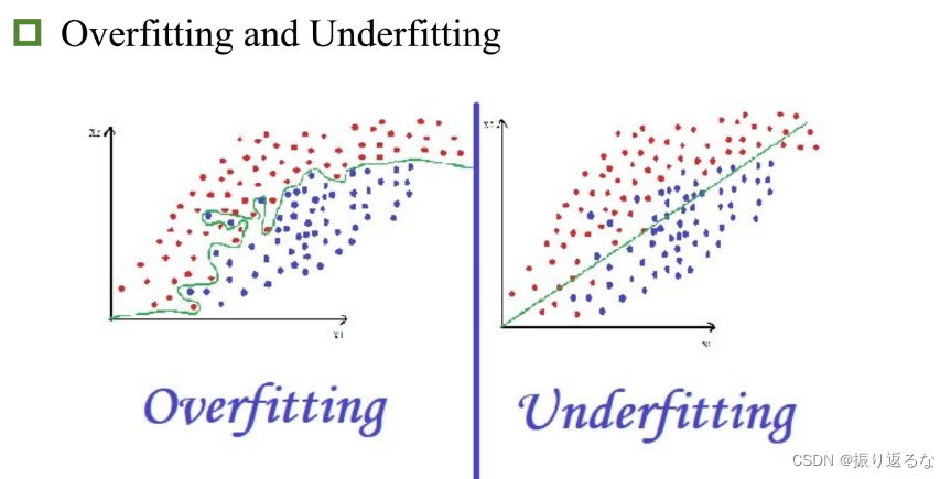
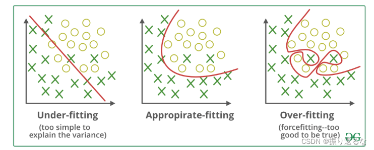
这张图很好地描述了过拟合和欠拟合地特点。
欠拟合学的太少,分类过于粗糙和简单。
过拟合学的太细,把细枝末节也包含在内,模型太过复杂。

Techniques to reduce underfitting:
•Increase model complexity
•Increase the number of features, performing feature engineering
•Remove noise from the data.
•Increase the number of epochs or increase the duration of training to get better results.
Techniques to reduce overfitting:
•Increase training data.
•Reduce model complexity.
•Early stopping during the training phase (have an eye over the loss over the training period as soon as loss begins to increase stop training).
•Ridge Regularization and Lasso Regularization(正则化)
•Use dropout for neural networks to tackle overfitting.
2、Evaluation Methods
Hold-out Method (留出法)
- 留出法(Hold-out Method): 直接将数据集D划分成两个互斥的集合,其中一个为训练集S,另一个作为测试集T,这称为“留出法”。
- 分层采样(stratified sampling): 在对数据集进行划分的时候,保留类别比例的采样方式称为“分层采样”。若对数据集D(包含500个正例,500个反例)则分层采样的到的训练集S(70%)应为350个正例,350个反例,测试集(30%)应为150个正例,150个反例。
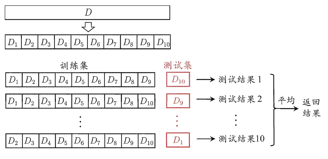
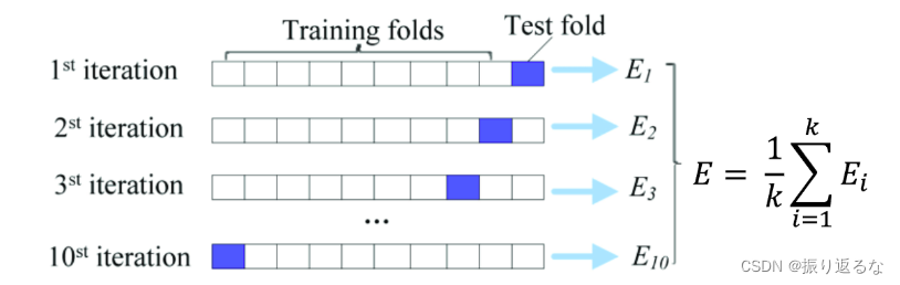
Cross Validation (交叉验证法)

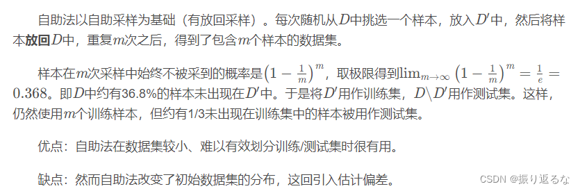
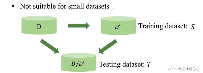
Bootstrapping(自助法)
Performance Measure(模型性能度量)
“性能度量(performance measure)”即衡量模型泛化能力的评价标准。
模型的“好坏”不仅取决于算法f和数据D,还决定于任务需求,而性能度量所反映的就是任务需求。
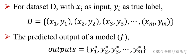
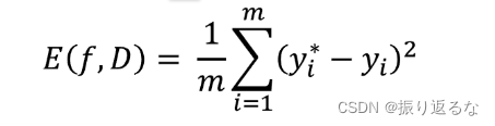
For regression tasks(回归任务):Mean Squared Error(均方差简称MSE)
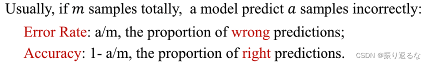
The classification task(分类): ErrorRate, Accuracy

Confusion Matrix 混淆矩阵
For binary classification tasks
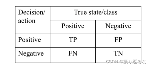
TP:预测类别为Positive,结果正确True。
TN:预测类别为Negative,结果正确True。
FN:预测类别为Negative,结果错误False。
FP:预测类别为Positive,结果错误False。

Precision也可以称为查准率,Recall也可以称为 查全率
P-R Curve: Precision-Recall
查准率和查全率是一对矛盾的度量。一般来说,查准率高时,查全率往往偏低;查全率高时,查准率往往偏低。通常只有在一些简单的任务中,才可能使得查准率和查全率都很高。
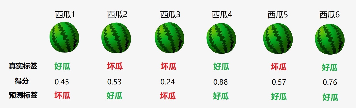
参考大佬的例子(https://blog.csdn.net/raelum/article/details/125041310):
假定阈值就是 0.5,我们的二分类器对于六个样例的打分情况如下:
我们根据这六个西瓜的得分将它们从高到低进行排序:
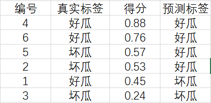
现在,我们从上往下遍历。对于第一行的样例,设它的得分 0.88为阈值,大于等于该阈值的预测为正例,小于该阈值的预测为反例,相应的结果如下:

计算可得查准率和查全率分别为 P = 1 , R = 0.33 。
对于第二行的样例,设它的得分 0.76为阈值,大于等于该阈值的预测为正例,小于该阈值的预测为反例,相应的结果如下:

计算可得查准率和查全率分别为 P = 1 , R = 0.67
以此类推,我们最终可以得到6(R,P)值。绘制P-R图:

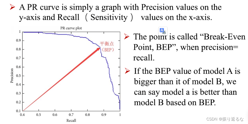
平衡点(Break-Even Point,简称BEP)就是这样一种度量,它是 P = R 时的取值。

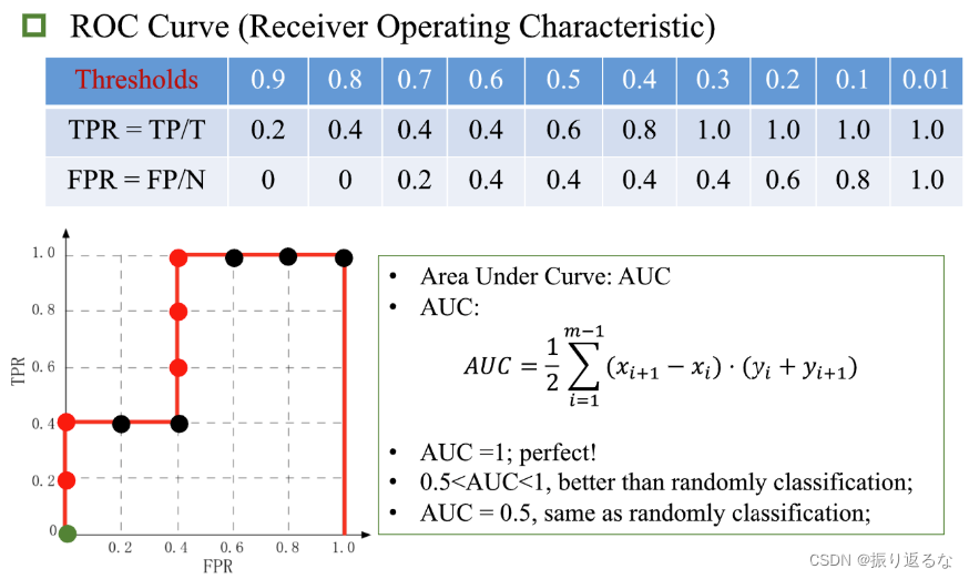
ROC Curve (Receiver Operating Characteristic 受试者工作特征)
此前我们已经提到,对m个样例的得分从高到低排序可以得到一个有序列表。在不同的应用任务中,我们可根据任务需求来设置不同的阈值(截断点)。若更重视查准率,则可在列表中靠前的位置进行截断;若更重视查全率,则可在列表中靠后的位置进行截断。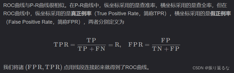
例子:
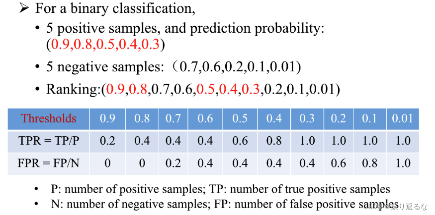
Thresholds :阈值。
在进行学习器的比较时,与P-R图相似,若一个学习器的ROC曲线被另一个学习器的曲线完全包住,则可断言后者的性能优于前者。如果两个学习器的ROC曲线发生交叉,那么我们就要比较ROC曲线下的面积,即AUC(Area Under roc Curve)