Model Selection & Evaluation

Model Selection & Evaluation

---

Agenda

1. Cross Validation
2. Hyperparameter Tuning
3. Model Evaluation
4. Model Persistance
5. Validation Curves
6. Learning Curves
7. 交叉验证
8. 超参数调整
9. 模型评估
10. 模型的持久性
11. 验证曲线
12. 学习曲线

---

Cross Validation交叉验证

• Simple models underfit.
• Accuracy for training data & validation data is not much different.
• But, accurcy ain’t that great.
• This situation is of low variance & high bias
• On moving towards complex models, accuracy improves.
• But, gap between accuracy on training data & validation data increases
• This situation is of high variance & low bias
• 简单模型的拟合度不足。
• 训练数据和验证数据的准确度没有太大区别。
• 但是，准确度没有那么高。
• 这种情况是低方差和高偏差。
• 在向复杂模型发展的过程中，准确度有所提高。
• 但是，训练数据和验证数据的准确性之间的差距会增加。
• 这种情况是高偏差和低偏差。

• We need to compare across models to find the best model.
• We need to compare across all hyper-parameters for a particular model.
• The data that is used for training should not be used for validation.
• The validation accuracy is the one that we claims
• 我们需要在不同模型之间进行比较，以找到最佳模型。
• 我们需要对一个特定模型的所有超参数进行比较。
• 用于训练的数据不应该被用于验证。
• 验证精度就是我们所声称的验证精度。

from sklearn.tree import DecisionTreeClassifier
from sklearn.datasets import load_digits
import matplotlib.pyplot as plt
%matplotlib inline

digits = load_digits()
plt.imshow(digits.images[0],cmap='gray')

from sklearn.model_selection import train_test_split
dt = DecisionTreeClassifier(max_depth=10)
trainX, testX, trainY, testY = train_test_split(digits.data, digits.target)
dt.fit(trainX,trainY)

DecisionTreeClassifier(class_weight=None, criterion='gini', max_depth=10,
                       max_features=None, max_leaf_nodes=None,
                       min_impurity_decrease=0.0, min_impurity_split=None,
                       min_samples_leaf=1, min_samples_split=2,
                       min_weight_fraction_leaf=0.0, presort=False,
                       random_state=None, splitter='best')

dt.score(testX,testY)

0.8355555555555556

dt.score(trainX,trainY)

0.9740163325909429

• Decreasing the complexity of model
• 降低模型的复杂性

dt = DecisionTreeClassifier(max_depth=7)
dt.fit(trainX,trainY)

DecisionTreeClassifier(class_weight=None, criterion='gini', max_depth=7,
                       max_features=None, max_leaf_nodes=None,
                       min_impurity_decrease=0.0, min_impurity_split=None,
                       min_samples_leaf=1, min_samples_split=2,
                       min_weight_fraction_leaf=0.0, presort=False,
                       random_state=None, splitter='best')

dt.score(testX,testY)

0.8155555555555556

dt.score(trainX,trainY)

0.8864142538975501

• Observation : With decrease in complexity the gap in training & validation accuracy also decreased
• 观察：随着复杂度的降低，训练和验证精度的差距也在缩小。

Cross Validation API交叉验证API

• Splits data into k parts.
• Use k - 1 parts for training the model
• Use kth part for validation
• Repeat the above steps multiple times to get a generalized behaviour
• 将数据分割成k个部分。
• 使用k-1部分来训练模型。
• 使用第K部分进行验证
• 重复上述步骤多次，得到一个通用的行为。

from sklearn.model_selection import cross_val_score

scores = cross_val_score(dt, digits.data, digits.target)

d:\Anaconda3\lib\site-packages\sklearn\model_selection\_split.py:1978: FutureWarning: The default value of cv will change from 3 to 5 in version 0.22. Specify it explicitly to silence this warning.
  warnings.warn(CV_WARNING, FutureWarning)

scores

array([0.68604651, 0.8096828 , 0.74161074])

scores.mean()

0.7457800181857993

Cross-validate Function : Scores for multiple matrices交叉验证函数：多个矩阵的分数

from sklearn.model_selection import cross_validate
scoring = ['precision_macro', 'recall_macro', 'accuracy']
results=cross_validate(dt, digits.data, digits.target, scoring=scoring, cv=5)
results

{'fit_time': array([0.01800108, 0.01200056, 0.01400089, 0.01300073, 0.01400089]),
 'score_time': array([0.00300026, 0.00300002, 0.00200009, 0.00300002, 0.00300002]),
 'test_precision_macro': array([0.7732771 , 0.71087424, 0.77524663, 0.78964348, 0.7585891 ]),
 'test_recall_macro': array([0.76278636, 0.66593093, 0.76876662, 0.77198413, 0.74553688]),
 'test_accuracy': array([0.76373626, 0.66574586, 0.76880223, 0.77310924, 0.74366197])}

for k, v in results.items():
    print(k,end=' ')
    print(v)

fit_time [0.01800108 0.01200056 0.01400089 0.01300073 0.01400089]
score_time [0.00300026 0.00300002 0.00200009 0.00300002 0.00300002]
test_precision_macro [0.7732771  0.71087424 0.77524663 0.78964348 0.7585891 ]
test_recall_macro [0.76278636 0.66593093 0.76876662 0.77198413 0.74553688]
test_accuracy [0.76373626 0.66574586 0.76880223 0.77310924 0.74366197]

results.keys()

dict_keys(['fit_time', 'score_time', 'test_precision_macro', 'test_recall_macro', 'test_accuracy'])

import pandas as pd
results=pd.DataFrame(results.values(),index=results.keys()).T

results

	fit_time	score_time	test_precision_macro	test_recall_macro	test_accuracy
0	0.018001	0.003	0.773277	0.762786	0.763736
1	0.012001	0.003	0.710874	0.665931	0.665746
2	0.014001	0.002	0.775247	0.768767	0.768802
3	0.013001	0.003	0.789643	0.771984	0.773109
4	0.014001	0.003	0.758589	0.745537	0.743662

Stratification for dealing with imbalanced Classes分层处理不平衡类的问题

• StratifiedKFold
  • Class frequencies are preserved in data splitting
• 分层KFold
  • 类频率在数据拆分中得到保留

import numpy as np

Y = np.append(np.ones(12),np.zeros(6))
X = np.ones((18,3))

from sklearn.model_selection import StratifiedKFold
skf = StratifiedKFold(n_splits=3)
list(skf.split(X,Y))

[(array([ 4,  5,  6,  7,  8,  9, 10, 11, 14, 15, 16, 17]),
  array([ 0,  1,  2,  3, 12, 13])),
 (array([ 0,  1,  2,  3,  8,  9, 10, 11, 12, 13, 16, 17]),
  array([ 4,  5,  6,  7, 14, 15])),
 (array([ 0,  1,  2,  3,  4,  5,  6,  7, 12, 13, 14, 15]),
  array([ 8,  9, 10, 11, 16, 17]))]

Y[[ 4,  5,  6,  7,  8,  9, 10, 11, 14, 15, 16, 17]]

array([1., 1., 1., 1., 1., 1., 1., 1., 0., 0., 0., 0.])

Hyperparameter Tuning 超参数调整

• Model parameters are learnt by learning algorithms based on data
• Hyper-parameters needs to be configured
• Hyper-parameters are data dependent & many times need experiments to find the best
• sklearn provides GridSerach for finding the best hyper-parameters

Exhaustive GridSearch穷尽的网格搜索

• Searches sequentially for all the configued params

• For all possible combinations

• 模型参数由学习算法根据数据学习算法来学习。

• 需要配置超参数。

• 超参数依赖于数据，很多时候需要通过实验来找到最佳的参数。

• sklearn提供了GridSerach，用于寻找最佳的超参数。

• 按顺序搜索所有配置的参数。

• 对于所有可能的组合

trainX, testX, trainY, testY = train_test_split(digits.data, digits.target)
dt = DecisionTreeClassifier()
from sklearn.model_selection import GridSearchCV
grid_search = GridSearchCV(dt, param_grid={'max_depth':range(5,30,5)}, cv=5)
grid_search.fit(digits.data,digits.target)

d:\Anaconda3\lib\site-packages\sklearn\model_selection\_search.py:814: DeprecationWarning: The default of the `iid` parameter will change from True to False in version 0.22 and will be removed in 0.24. This will change numeric results when test-set sizes are unequal.
  DeprecationWarning)





GridSearchCV(cv=5, error_score='raise-deprecating',
             estimator=DecisionTreeClassifier(class_weight=None,
                                              criterion='gini', max_depth=None,
                                              max_features=None,
                                              max_leaf_nodes=None,
                                              min_impurity_decrease=0.0,
                                              min_impurity_split=None,
                                              min_samples_leaf=1,
                                              min_samples_split=2,
                                              min_weight_fraction_leaf=0.0,
                                              presort=False, random_state=None,
                                              splitter='best'),
             iid='warn', n_jobs=None, param_grid={'max_depth': range(5, 30, 5)},
             pre_dispatch='2*n_jobs', refit=True, return_train_score=False,
             scoring=None, verbose=0)

grid_search.best_params_

{'max_depth': 20}

grid_search.best_score_

0.7868670005564831

grid_search.best_estimator_

DecisionTreeClassifier(class_weight=None, criterion='gini', max_depth=20,
                       max_features=None, max_leaf_nodes=None,
                       min_impurity_decrease=0.0, min_impurity_split=None,
                       min_samples_leaf=1, min_samples_split=2,
                       min_weight_fraction_leaf=0.0, presort=False,
                       random_state=None, splitter='best')

RandomizedSearch随机搜索

• Unlike GridSearch, not all parameters are tried & tested
• But rather a fixed number of parameter settings is sampled from the specified distributions.

Comparing GridSearch and RandomSearchCV

• 与GridSearch不同，不是所有的参数都是经过测试的。
• 而是从指定的分布中抽出一个固定数量的参数设置。

比较GridSearch和RandomSearchCV。

from time import time

#randint is an intertor for generating numbers between range specified
from scipy.stats import randint
X = digits.data
Y = digits.target

from sklearn.ensemble import RandomForestClassifier
from sklearn.model_selection import RandomizedSearchCV, GridSearchCV

# specify parameters and distributions to sample from
param_dist = {"max_depth": [3, None],
              "max_features": randint(1,11),
              "min_samples_split": randint(2, 11),
              "bootstrap": [True, False],
              "criterion": ["gini", "entropy"]}

param_dist

{'max_depth': [3, None],
 'max_features': <scipy.stats._distn_infrastructure.rv_frozen at 0xf179248>,
 'min_samples_split': <scipy.stats._distn_infrastructure.rv_frozen at 0xf1793c8>,
 'bootstrap': [True, False],
 'criterion': ['gini', 'entropy']}

rf = RandomForestClassifier(n_estimators=20)
n_iter_search = 20
random_search = RandomizedSearchCV(rf, param_distributions=param_dist,
                                   n_iter=n_iter_search, cv=5)

start = time()
random_search.fit(X, Y)
print("RandomizedSearchCV took %.2f seconds for %d candidates"
      " parameter settings." % ((time() - start), n_iter_search))

RandomizedSearchCV took 4.52 seconds for 20 candidates parameter settings.


d:\Anaconda3\lib\site-packages\sklearn\model_selection\_search.py:814: DeprecationWarning: The default of the `iid` parameter will change from True to False in version 0.22 and will be removed in 0.24. This will change numeric results when test-set sizes are unequal.
  DeprecationWarning)

random_search.best_score_

0.9365609348914858

param_grid = {"max_depth": [3, None],
              "max_features": [1, 3, 10],
              "min_samples_split": [2, 3, 10],
              "bootstrap": [True, False],
              "criterion": ["gini", "entropy"]}

# run grid search
grid_search = GridSearchCV(rf, param_grid=param_grid, cv=5)
start = time()
grid_search.fit(X, Y)

print("GridSearchCV took %.2f seconds for %d candidate parameter settings."
      % (time() - start, len(grid_search.cv_results_['params'])))

GridSearchCV took 15.34 seconds for 72 candidate parameter settings.


d:\Anaconda3\lib\site-packages\sklearn\model_selection\_search.py:814: DeprecationWarning: The default of the `iid` parameter will change from True to False in version 0.22 and will be removed in 0.24. This will change numeric results when test-set sizes are unequal.
  DeprecationWarning)

grid_search.best_score_

0.9354479688369505

• GridSearch & RandomizedSearch can fine tune hyper-parameters of transformers as well when part of pipeline
• GridSearch和RandomizedSearch可以微调变压器的超参数，当管道的一部分时，也可以微调变压器的超参数。

Model Evaluation模型评估

• Three different ways to evaluate quality of model prediction
  • score method of estimators, a default method is configured .i.e r2_score for regression, accuracy for classification
  • Model evalutaion tools like cross_validate or cross_val_score also returns accuracy
  • Metrices module is rich with various prediction error calculation techniques
• 评价模型预测质量的三种不同方法
  • 估计器的得分方法，默认配置了一种方法，即r2_score用于回归，准确度用于分类。
  • 模型评估工具如cross_validate或cross_val_score等模型评估工具也会返回精度。
  • Metrices模块具有丰富的各种预测误差计算技术。

trainX, testX, trainY, testY = train_test_split(X,Y)
rf.fit(trainX, trainY)

RandomForestClassifier(bootstrap=True, class_weight=None, criterion='gini',
                       max_depth=None, max_features='auto', max_leaf_nodes=None,
                       min_impurity_decrease=0.0, min_impurity_split=None,
                       min_samples_leaf=1, min_samples_split=2,
                       min_weight_fraction_leaf=0.0, n_estimators=20,
                       n_jobs=None, oob_score=False, random_state=None,
                       verbose=0, warm_start=False)

• Technique 1 - Using score function
• 技巧一----使用评分函数

rf.score(testX,testY)

0.9577777777777777

• Technique 2 - Using cross_val_score as discussed above
• 技巧2 - 使用上文讨论过的cross_val_score

cross_val_score(rf,X,Y,cv=5)

array([0.92307692, 0.90055249, 0.93871866, 0.94677871, 0.88169014])

Cancer prediction sample for understanding metrices癌症预测样本了解度量衡的癌症预测样本

from sklearn.datasets import load_breast_cancer
dt = DecisionTreeClassifier()
cancer_data = load_breast_cancer()
trainX, testX, trainY, testY = train_test_split(cancer_data.data, cancer_data.target)

dt.fit(trainX,trainY)

DecisionTreeClassifier(class_weight=None, criterion='gini', max_depth=None,
                       max_features=None, max_leaf_nodes=None,
                       min_impurity_decrease=0.0, min_impurity_split=None,
                       min_samples_leaf=1, min_samples_split=2,
                       min_weight_fraction_leaf=0.0, presort=False,
                       random_state=None, splitter='best')

pred = dt.predict(testX)

Technique 3 - Using metrices使用衡量指标

Classfication metrices分类衡量指标

• Accuracy Score - Correct classification vs ( Correct classification + Incorrect Classification )
• 准确率得分 - 正确分类与（正确分类+不正确分类）的比较

from sklearn import metrics
metrics.accuracy_score(y_pred=pred, y_true=testY)

0.9300699300699301

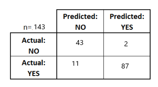
• Confusion Matrix - Shows details of classification inclusing TP,FP,TN,FN
  • True Positive (TP), Actual class is 1 & prediction is also 1
  • True Negative (TN), Actual class is 0 & prediction is also 0
  • False Positive (FP), Acutal class is 0 & prediction is 1
  • False Negative (FN), Actual class is 1 & prediction is 0

confusion_result=metrics.confusion_matrix(y_pred=pred, y_true=testY, labels=[0,1])
confusion_result

array([[60,  6],
       [ 4, 73]], dtype=int64)

tp=confusion_result[1][1]
tn=confusion_result[0][0]
fp=confusion_result[0][1]
fn=confusion_result[1][0]

• Precision Score精确度得分
  • Ability of a classifier not to label positive if the sample is negative
  • Claculated as TP/(TP+FP)
  • We don’t want a non-spam mail to be marked as spam
  • 如果样本为负值，分类器不标记正值的能力
  • 按TP/(TP+FP)的形式计算
  • 我们不希望非垃圾邮件被标记为垃圾邮件。

precision_result=tp/(tp+fp)
precision_result

0.9240506329113924

metrics.precision_score(y_pred=pred, y_true=testY)

0.9240506329113924

• Recall Score召回率
  • Ability of classifier to find all positive samples
  • It’s ok to predict patient tumor to be cancer so that it undergoes more test
  • But it is not ok to miss a cancer patient without further analysis
  • 找到所有阳性样本的能力
  • 預測病人的腫瘤是癌症是可以的，所以要多做一些測試
  • 但如果没有进一步的分析，错过了癌症患者也是不行的。

metrics.recall_score(y_pred=pred, y_true=testY)

0.948051948051948

• F1 score
  • Weighted average of precision & recall

metrics.f1_score(y_pred=pred, y_true=testY)

0.9358974358974359

• ROC & AUC

House Price Prediction - Understanding matrices

from sklearn.datasets import california_housing
house_data = california_housing.fetch_california_housing()
from sklearn.linear_model import LinearRegression
lr = LinearRegression()
lr.fit(house_data.data, house_data.target)

LinearRegression(copy_X=True, fit_intercept=True, n_jobs=None, normalize=False)

pred = lr.predict(house_data.data)

Matrices for Regression

• mean squared error
  • Sum of squares of difference between expected value & actual value

metrics.mean_squared_error(y_pred=pred, y_true=house_data.target)

0.5243209861846071

• mean absolute error
  • Sum of abs of difference between expected value & actual value

metrics.mean_absolute_error(y_pred=pred, y_true=house_data.target)

0.5311643817546461

• r2 score

  • Returns accuracy of model in the scale of 0 & 1
  • It measures goodness of fit for regression models
  • Calculated as = (variance explained by the model)/(Total variance)
  • High r2 means target is close to prediction
  

metrics.r2_score(y_pred=pred, y_true=house_data.target)

0.6062326851998051

Metrices for Clustering 用于聚类的衡量指标

• Two forms of evaluation
• supervised, which uses a ground truth class values for each sample.
  • completeness_score
  • homogeneity_score
• unsupervised, which measures the quality of model itself
  • silhoutte_score
  • calinski_harabaz_score
• 两种评价形式
• 监督的，它为每个样本使用了一个地面真值类的值。
  • 完整度_score
  • 同质性分数
• 无监督，衡量模型本身的质量
  • silhoutte_score
  • calinski_harabaz_score

completeness_score

• A clustering result satisfies completeness if all the data points that are members of a given class are elements of the same cluster.
• Accuracy is 1.0 if data belonging to same class belongs to same cluster, even if multiple classes belongs to same cluster

from sklearn.metrics.cluster import completeness_score

completeness_score( labels_true=[10,10,11,11],labels_pred=[1,1,0,0])

1.0

• The acuracy is 1.0 because all the data belonging to same class belongs to same cluster

completeness_score( labels_true=[11,22,22,11],labels_pred=[1,0,1,1])

0.3836885465963443

• The accuracy is .3 because class 1 - [11,22,11], class 2 - [22]

print(completeness_score([10, 10, 11, 11], [0, 0, 0, 0]))

1.0

homogeneity_score

• A clustering result satisfies homogeneity if all of its clusters contain only data points which are members of a single class.

from sklearn.metrics.cluster import homogeneity_score

homogeneity_score([0, 0, 1, 1], [1, 1, 0, 0])

1.0

homogeneity_score([0, 0, 1, 1], [0, 1, 2, 3])

0.9999999999999999

homogeneity_score([0, 0, 0, 0], [1, 1, 0, 0])

1.0

• Same class data is broken into two clusters

silhoutte_score

• The Silhouette Coefficient is calculated using the mean intra-cluster distance (a) and the mean nearest-cluster distance (b) for each sample.
• The Silhouette Coefficient for a sample is (b - a) / max(a, b). To clarify, b is the distance between a sample and the nearest cluster that the sample is not a part of.

Selecting the number of clusters with silhouette analysis on KMeans clustering

from sklearn.datasets import make_blobs
X, Y = make_blobs(n_samples=500,
                  n_features=2,
                  centers=4,
                  cluster_std=1,
                  center_box=(-10.0, 10.0),
                  shuffle=True,
                  random_state=1)

plt.scatter(X[:,0],X[:,1],s=10)

range_n_clusters = [2, 3, 4, 5, 6]

from sklearn.cluster import KMeans
from sklearn.metrics import silhouette_score

for n_cluster in range_n_clusters:
    kmeans = KMeans(n_clusters=n_cluster)
    kmeans.fit(X)
    labels = kmeans.predict(X)
    print (n_cluster, silhouette_score(X,labels))

2 0.7049787496083262
3 0.5882004012129721
4 0.6505186632729437
5 0.5746932321727457
6 0.49417400746431644

• The best number of clusters is 2

calinski_harabaz_score

• The score is defined as ratio between the within-cluster dispersion and the between-cluster dispersion.

from sklearn.metrics import calinski_harabaz_score

for n_cluster in range_n_clusters:
    kmeans = KMeans(n_clusters=n_cluster)
    kmeans.fit(X)
    labels = kmeans.predict(X)
    print (n_cluster, calinski_harabaz_score(X,labels))

2 1604.112286409658
3 1809.991966958033
4 2704.4858735121097
5 2281.91411035916
6 2040.6320809618921

Model Persistance

• Model training is an expensive process
• It is desireable to save the model for future reuse
• using pickle & joblib this can be achieved
• 模型培训是一个昂贵的过程
• 希望将模型保存下来，以便将来再利用。
• 使用pickle和joblib可以实现这个功能

import pickle
s = pickle.dumps(dt)
pickle.loads(s)

DecisionTreeClassifier(class_weight=None, criterion='gini', max_depth=None,
                       max_features=None, max_leaf_nodes=None,
                       min_impurity_decrease=0.0, min_impurity_split=None,
                       min_samples_leaf=1, min_samples_split=2,
                       min_weight_fraction_leaf=0.0, presort=False,
                       random_state=None, splitter='best')

type(s)

bytes

• joblib is better extension of pickle
• Doesn’t convert into string

from sklearn.externals import joblib
joblib.dump(dt, 'dt.joblib')

['dt.joblib']

• Loading the file back into model

dt = joblib.load('dt.joblib')
dt

DecisionTreeClassifier(class_weight=None, criterion='gini', max_depth=None,
                       max_features=None, max_leaf_nodes=None,
                       min_impurity_decrease=0.0, min_impurity_split=None,
                       min_samples_leaf=1, min_samples_split=2,
                       min_weight_fraction_leaf=0.0, presort=False,
                       random_state=None, splitter='best')

Validation Curves验证曲线

• To validate a model, we need a scoring function.
• Create a grid of possible hyper-prameter configuration.
• Select the hyper-parameter which gives the best score
• 要验证一个模型，我们需要一个评分函数。
• 创建一个可能的超参数配置的网格。
• 选择一个能给出最佳得分的超参数。

from sklearn.model_selection import validation_curve

param_range = np.arange(1, 50, 2)

train_scores, test_scores = validation_curve(RandomForestClassifier(), 
                                             digits.data, 
                                             digits.target, 
                                             param_name="n_estimators", 
                                             param_range=param_range,
                                             cv=3, 
                                             scoring="accuracy", 
                                             n_jobs=-1)

train_mean = np.mean(train_scores, axis=1)
train_std = np.std(train_scores, axis=1)

test_mean = np.mean(test_scores, axis=1)
test_std = np.std(test_scores, axis=1)

plt.plot(param_range, train_mean, label="Training score", color="black")
plt.plot(param_range, test_mean, label="Cross-validation score", color="dimgrey")

plt.title("Validation Curve With Random Forest")
plt.xlabel("Number Of Trees")
plt.ylabel("Accuracy Score")
plt.tight_layout()
plt.legend(loc="best")
plt.show()

6. Learning Curves

• Learning curves shows variation in training & validation score on increasing the number of samples

from sklearn.model_selection import learning_curve