前几天女朋友有个R语言的大作业,寻求了本人的帮助,在此记录一下,也希望能帮到你。其中部分内容来自于她的报告。
数据集
数据集使用Yale_32x32.mat作为示例,耶鲁大学人脸数据库,均为像素为32×32的灰度图像。
包含15个人的人脸,每个人有不同表情、姿态和光照下的11张人脸图像,共165张图片。

使用R语言读取得到:
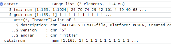
fea是特征,也就是像素值,gnd是标签,代表属于第几个人的照片。
nnet的使用
以下是官方的介绍和例程:
Fit Neural Networks
Description
Fit single-hidden-layer neural network, possibly with skip-layer connections.

Usage
nnet(x, ...)

## S3 method for class 'formula'
nnet(formula, data, weights, ...,
     subset, na.action, contrasts = NULL)

## Default S3 method:
nnet(x, y, weights, size, Wts, mask,
     linout = FALSE, entropy = FALSE, softmax = FALSE,
     censored = FALSE, skip = FALSE, rang = 0.7, decay = 0,
     maxit = 100, Hess = FALSE, trace = TRUE, MaxNWts = 1000,
     abstol = 1.0e-4, reltol = 1.0e-8, ...)
Arguments
formula
A formula of the form class ~ x1 + x2 + ...

x
matrix or data frame of x values for examples.

y
matrix or data frame of target values for examples.

weights
(case) weights for each example – if missing defaults to 1.

size
number of units in the hidden layer. Can be zero if there are skip-layer units.

data
Data frame from which variables specified in formula are preferentially to be taken.

subset
An index vector specifying the cases to be used in the training sample. (NOTE: If given, this argument must be named.)

na.action
A function to specify the action to be taken if NAs are found. The default action is for the procedure to fail. An alternative is na.omit, which leads to rejection of cases with missing values on any required variable. (NOTE: If given, this argument must be named.)

contrasts
a list of contrasts to be used for some or all of the factors appearing as variables in the model formula.

Wts
initial parameter vector. If missing chosen at random.

mask
logical vector indicating which parameters should be optimized (default all).

linout
switch for linear output units. Default logistic output units.

entropy
switch for entropy (= maximum conditional likelihood) fitting. Default by least-squares.

softmax
switch for softmax (log-linear model) and maximum conditional likelihood fitting. linout, entropy, softmax and censored are mutually exclusive.

censored
A variant on softmax, in which non-zero targets mean possible classes. Thus for softmax a row of (0, 1, 1) means one example each of classes 2 and 3, but for censored it means one example whose class is only known to be 2 or 3.

skip
switch to add skip-layer connections from input to output.

rang
Initial random weights on [-rang, rang]. Value about 0.5 unless the inputs are large, in which case it should be chosen so that rang * max(|x|) is about 1.

decay
parameter for weight decay. Default 0.

maxit
maximum number of iterations. Default 100.

Hess
If true, the Hessian of the measure of fit at the best set of weights found is returned as component Hessian.

trace
switch for tracing optimization. Default TRUE.

MaxNWts
The maximum allowable number of weights. There is no intrinsic limit in the code, but increasing MaxNWts will probably allow fits that are very slow and time-consuming.

abstol
Stop if the fit criterion falls below abstol, indicating an essentially perfect fit.

reltol
Stop if the optimizer is unable to reduce the fit criterion by a factor of at least 1 - reltol.

...
arguments passed to or from other methods.

Details
If the response in formula is a factor, an appropriate classification network is constructed; this has one output and entropy fit if the number of levels is two, and a number of outputs equal to the number of classes and a softmax output stage for more levels. If the response is not a factor, it is passed on unchanged to nnet.default.

Optimization is done via the BFGS method of optim.

Value
object of class "nnet" or "nnet.formula". Mostly internal structure, but has components

wts
the best set of weights found

value
value of fitting criterion plus weight decay term.

fitted.values
the fitted values for the training data.

residuals
the residuals for the training data.

convergence
1 if the maximum number of iterations was reached, otherwise 0.

References
Ripley, B. D. (1996) Pattern Recognition and Neural Networks. Cambridge.

Venables, W. N. and Ripley, B. D. (2002) Modern Applied Statistics with S. Fourth edition. Springer.

See Also
predict.nnet, nnetHess

Examples
# use half the iris data
ir <- rbind(iris3[,,1],iris3[,,2],iris3[,,3])
targets <- class.ind( c(rep("s", 50), rep("c", 50), rep("v", 50)) )
samp <- c(sample(1:50,25), sample(51:100,25), sample(101:150,25))
ir1 <- nnet(ir[samp,], targets[samp,], size = 2, rang = 0.1,
            decay = 5e-4, maxit = 200)
test.cl <- function(true, pred) {
    true <- max.col(true)
    cres <- max.col(pred)
    table(true, cres)
}
test.cl(targets[-samp,], predict(ir1, ir[-samp,]))


# or
ird <- data.frame(rbind(iris3[,,1], iris3[,,2], iris3[,,3]),
        species = factor(c(rep("s",50), rep("c", 50), rep("v", 50))))
ir.nn2 <- nnet(species ~ ., data = ird, subset = samp, size = 2, rang = 0.1,
               decay = 5e-4, maxit = 200)
table(ird$species[-samp], predict(ir.nn2, ird[-samp,], type = "class"))
接下来介绍一下本人的使用:
nnet <- nnet(train, targets.train, size = 10, rang = 1, decay = 1e-3,
                maxit = 200, MaxNWts=30000)
其中的train是指训练的数据,也就是归一化后的像素值, targets.train是与train对应的独热码标签,size是隐藏层的层数,rang是训练集的数据数值范围,decay是权值衰减系数,maxit是最大迭代次数,MaxNWts好像是最大参数量。
独热码转换示例:

完整代码
完整的代码如下:
library("R.matlab")


path<-("F:\\R_language")
pathname <- file.path(path, "Yale_32x32.mat")
datatr <- readMat(pathname)

feattr=datatr[[1]]
feattr = feattr / 127.5 - 1 #归一化
datatrnum=datatr[[2]]
result <- array(c(0),dim = c(165,15))# 转化为独热码
cnt <- 1
repeat {
  result[cnt, datatrnum[cnt, 1]] <- 1
  cnt <- cnt+1

  if(cnt > 165) {
    break
  }
}


set.seed(521)
##70%的数据集作为训练模型
samp <- c(sample(1:165,135))
train <- feattr[samp,]
targets.train <- result[samp,]
validation <- feattr[-samp,]
targets.validation <- result[-samp,]
library(nnet)
nnet <- nnet(train, targets.train, size = 10, rang = 1,decay = 5e-4,
                maxit = 200, MaxNWts=30000)
summary(nnet)

true = max.col(true)
cres = max.col(pred)
table(true, cres)
}
test.cl(targets.validation, predict(nnet, validation))
cres = max.col(predict(nnet, validation))
true = max.col(targets.validation)
plot(x=cres,y=true,col="red",xlab="预测值",ylab="真实值")
cnt =1
correct = 0
repeat {
if(cres[cnt]==true[cnt])
{
correct <- correct + 1
}
cnt <- cnt+1
if(cnt > length(cres)) {
break
}
}
correct/length(cres)#正确率
训练过程和结果
由于数据是随机抽取70%作为训练集,所以每次的训练集和测试集都不太相同,所以结果也会不同。
训练200个iter,训练过程中的loss如下:
 weights:  10415
initial  value 432.348356
iter  10 value 135.657129
iter  20 value 131.287453
iter  30 value 127.033601
iter  40 value 118.414307
iter  50 value 111.639129
iter  60 value 106.634401
iter  70 value 99.618272
iter  80 value 95.067623
iter  90 value 91.453289
iter 100 value 88.281143
iter 110 value 77.366638
iter 120 value 57.478618
iter 130 value 50.865985
iter 140 value 46.196341
iter 150 value 44.470719
iter 160 value 41.549106
iter 170 value 36.746992
iter 180 value 35.089741
iter 190 value 33.031845
iter 200 value 31.085787
final  value 31.085787
stopped after 200 iterations
进行测试后得到的混淆矩阵如下:

点状图:

以及当前正确率:
 >correct/length(cres)#正确率
[1] 0.5
结论
nnet的使用相比pytorch来说要容易上手的多,但是也注定只能处理简单的数据,对于高维数据(图片)来说模型的学习能力肯定不行,能够设置的参数也较少,也不能使用GPU进行训练,训练速度较慢。用在简单的数据拟合中效果应该还行,也方便上手。