80 R实现BP神经网络与参数调优

1 清理环境与准备

################nnet packages single hidden layer BP neural network###################################
##----------------------data loading and cleaning-----------------------------
#clean up enviroment variables loading Sonar, Mines vs. Rocks data
rm(list=ls())
#install.packages("mlbench")
library(mlbench)
data(Sonar)

确定y变量

# Redefine factor level
levels(Sonar$Class)<-c(0,1)

2 确定测试集与训练集

#random sampling
set.seed(1221)
select<-sample(1:nrow(Sonar),nrow(Sonar)*0.7)
train<-Sonar[select,]
test<-Sonar[-select,]

# standardized data
train[,1:60]=scale(train[,1:60])
test[,1:60]=scale(test[,1:60])

3 使用nnet包与参数说明

##---------------------Implementation of BP neural network using packet------------------------
#install.packages("nnet")
library(nnet)
mynnet<-nnet(Class~., linout =F,size=14, decay=0.0076, maxit=200, 
             data = train)
#linout judge whether the output is linear
# size is Number of nodes 
#decay is attenuation rate
#decay and learning rate are similar
#Maximum number of iterations

4 结果评估

##model predict
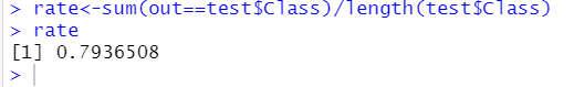
out<-predict(mynnet, test) 
out[out<0.5]=0
out[out>=0.5]=1
#test$Class=ifelse(test$Class=="M",1,0)
##calculation accuracy
rate<-sum(out==test$Class)/length(test$Class)
rate

5 绘制ROC曲线

####Predict on the training set and test set respectively
##The construction of ROC curve function ROC () is convenient.
##Note that this function will add columns to the data frame called
ROC<-function(model,train,test,objcolname,ifplot=TRUE){
  library(ROCR,quietly = T)
  train$p<-predict(model, train) 
  test$p<-predict(model, test) 
  
  predTr <- prediction(train$p, train[,objcolname])
  perfTr <- performance(predTr,"tpr","fpr")
  
  predTe <- prediction(test$p, test[,objcolname])
  perfTe <- performance(predTe,"tpr","fpr")
  
  tr_auc<-round(as.numeric(performance(predTr,'auc')@y.values),3)
  te_auc<-round(as.numeric(performance(predTe,'auc')@y.values),3)
  
  if(ifplot==T){
    plot(perfTr,col='green',main="ROC of Models")
    plot(perfTe, col='black',lty=2,add=TRUE);
    abline(0,1,lty=2,col='red')
    
    tr_str<-paste("Tran-AUC:",tr_auc,sep="")
    legend(0.3,0.45,c(tr_str),2:8)
    te_str<-paste("Test-AUC:",te_auc,sep="")
    legend(0.3,0.25,c(te_str),2:8)
  }
  auc<-data.frame(tr_auc,te_auc)
  return(auc)
}
ROC(model=mynnet,train=train,test=test,objcolname="Class",ifplot=T)

6 循环调整参数

############################Adjusting parameters########################################


##The predictive variables of the input data must be binary. And all variables only include model input and output variables.
##When adjusting parameters, if there are too many variables, the size should not be too large.
##Build the parameter adjustment function network().
network<-function(formula,data,size,adjust,decay=0,maxit=200,scale=TRUE,
                  samplerate=0.7,seed=1,linout=FALSE,ifplot=TRUE){
  library(nnet)
  ##The specification output variable is 0,1
  yvar<-colnames(data)==(all.vars(formula)[1])
  levels(data[,yvar])<-c(0,1)
  ##Establish training set and test set by sampling
  set.seed(seed)
  select<-sample(1:nrow(data),nrow(data)*samplerate)
  train=data[select,]
  test=data[-select,]
  ##Standardize according to given judgment
  if(scale==T){
    xvar<-colnames(data)!=(all.vars(formula)[1])
    train[,xvar]=scale(train[,xvar])
    test[,xvar]=scale(test[,xvar])
  }
  ##Recycle NNET training parameters
  obj<-eval(parse(text = adjust))
  auc<-data.frame()
  for(i in obj){
    if(adjust=="size"){
      mynnet<-nnet(formula,size=i,linout=linout,decay=decay,
                   maxit=maxit,trace=FALSE,data=train)
    }
    else if(adjust=="decay"){
      mynnet<-nnet(formula,size=size,linout=linout,decay=i,
                   maxit=maxit,trace=FALSE,data=train)
    }
    ##Call the previous roc() to get the AUC value of the corresponding parameterֵ
    objcolname<-all.vars(formula)[1]
    auc0<-ROC(model=mynnet,train=train,test=test,
              objcolname=objcolname,ifplot=F)
    ##Output data frames corresponding to different values of specified parameters
    out<-data.frame(i,auc0)
    auc<-rbind(auc,out)
  }
  
  names(auc)<-c(adjust,"Train_auc","Test_auc")
  # if(ifplot==T){
  #   library(plotrix)
  #   # twoord.plot(auc1[,1] , auc1$Train_auc , auc1[,1] , auc1$Test_auc , lcol=4 , rcol=2 , xlab=adjust , 
  #   #             ylab="Train_auc" , rylab="Test_auc" , type=c("l","b"),lab=c(15,5,10))
  # }
  return(auc)
}
auc<-network(Class~.,data=Sonar,size=1:16,adjust="size",
             decay=0.0001,maxit=200,scale=T)
which(auc$Test_auc==max(auc$Test_auc))
auc<-network(Class~.,data=Sonar,size=14,adjust="decay",
             decay=c(0,seq(0.0001,0.01,0.0003)),maxit=200)


plot(auc$decay,auc$Train_auc,ylim=c(0.8,1))
lines(auc$decay,auc$Train_auc)
points(auc$decay,auc$Test_auc)
lines(auc$decay,auc$Test_auc)


# #根据中左侧纵坐标是训练集 auc 值的变化，对应直线，右侧纵坐标是测试集对应点线。可见 size
# 大于 3 时就可以对训练集很好的拟合，而当 size 等于 14 是测试集的 ROC 指标较高，故这里我们选
# 取 size=14。
# 选取 size 后对指定一系列 decay 数值进行比较，这里选择的是从 0.0001 到 0.01 的等差数列差值
# 是 0.0003，同时包括 0。得到的结果如下：（运行时间较长， decay 的范围可以选取多个区间比较）

## according to the change of AUC value of the training set, the left ordinate corresponds to the straight line, and the right ordinate corresponds to the point line of the test set. Visible size
#When it is greater than 3, the training set can be well fitted. When the size is equal to 14, the ROC index of the test set is high, so we choose here
#Take size = 14.
#Select size and compare the specified series of decimal values. Here, select the difference of the arithmetic sequence from 0.0001 to 0.01
#Is 0.0003, including 0. The results are as follows: (the running time is long, and multiple intervals can be selected for the range of decay)