2022宁夏杯B题思路分析+代码（大学生就业问题分析）

2022宁夏杯B题完整题目：

链接：https://pan.baidu.com/s/1aClw5k-Ux-17rckTIRWrdg?pwd=1234

提取码：1234

一、题目

大学生就业问题一直是社会关注的焦点。据此前教育部新闻发布会通报， 2022 届高校毕业生规模达 1076 万人，首次突破 1000 万人，规模和增量均创下 了历史新高。同时受市场环境和疫情等因素的影响，就业压力较大。大学生就业 呈现出哪些特征和趋势呢？在众多就业的学生中，是什么样的因素决定了部分学 生在众多的竞争中获得了薪水不同的工作？这些因素可能包括大学的成绩、本身 的技能、大学与工业中心的接近程度、拥有的专业化程度、特定行业的市场条件等。 据悉，印度共有 6214 所工程和技术院校，其中约有 290 万名学生。每年平 均有 150 万学生获得工程学学位，但由于缺乏从事技术工作所需的技能，只有不 到 20% 的 学 生 在 其 核 心 领 域 找 到 工 作 。 附 件 （https://www.datafountain.cn/datasets/4955）给出了印度工程类专业毕业生就业的工资水平和各因素情况表。

根据附件数据结合其他资料研究：

(1) 分析影响高校工程类专业毕业生就业的主要因素。
(2) 根据附件一建立模型，刻画工程类专业毕业生薪水和各因素的关系。
(3) 根据以上的分析，对我国高校工程类专业学生培养是否有一定的启迪？ 如果有，请为你所在的高校写一份咨询建议。

属性	说明
ID	用于识别候选人的唯一ID
薪金	向候选人提供的年度CTC（以INR为单位）
性别	候选人的性别
DOB	候选人的出生日期
10％	在10年级考试中获得的总成绩
10board	10年级时遵循其课程的校务委员会
12毕业	毕业年份-高中
12％	在12年级考试中获得的总成绩
12board	候选人遵循其课程的校务委员会
CollegeID	唯一ID，用于标识候选人为其大学就读的大学/学院
CollegeTier	每所大学都被标注为1或2。标注是根据该学院/大学学生获得的平均AMCAT分数计算得出的。平均分数高于阈值的大学被标记为1，其他被标记为2。
学位	候选人获得/追求的学位
专业化	候选人追求的专业化
CollegeGPA	毕业时的GPA总计
CollegeCityID	唯一的ID，用于标识学院所在的城市。
CollegeCityTier	学院所在城市的层。这是根据城市人口进行注释的。
CollegeState	学院所在州的名称
毕业年份	毕业年份（学士学位）
英语	AMCAT英语部分中的分数
逻辑	在AMCAT逻辑能力部分中得分
数量	在AMCAT的“定量能力”部分中得分
域	AMCAT域模块中的分数
ComputerProgramming	AMCAT的“计算机编程”部分中的得分
ElectronicsAndSemicon	AMCAT的“电子和半导体工程”部分得分
计算机科学	在AMCAT的“计算机科学”部分中得分
MechanicalEngg	AMCAT机械工程部分中的得分
ElectricalEngg	AMCAT的电气工程部分中的得分
TelecomEngg	AMCAT的“电信工程”部分中的得分
CivilEngg	AMCAT的“土木工程”部分中的得分
尽职调查	AMCAT人格测验之一的分数
一致性	AMCAT人格测验之一的分数
外向性	AMCAT人格测验之一的分数
营养疗法	AMCAT人格测验之一的分数
开放性到经验	分数在AMCAT的个性测试的部分之一

二、数据预处理

• 目标变量：Salary（薪资）。
• 自变量（特征变量）：除了Salary之外的其他变量。

import pandas as pd 
import numpy as np 
data=pd.read_csv('B题附件.csv')
data.info()

<class 'pandas.core.frame.DataFrame'>
RangeIndex: 2998 entries, 0 to 2997
Data columns (total 34 columns):
 #   Column                 Non-Null Count  Dtype  
---  ------                 --------------  -----  
 0   ID                     2998 non-null   int64  
 1   Gender                 2998 non-null   object 
 2   DOB                    2998 non-null   object 
 3   10percentage           2998 non-null   float64
 4   10board                2998 non-null   object 
 5   12graduation           2998 non-null   int64  
 6   12percentage           2998 non-null   float64
 7   12board                2998 non-null   object 
 8   CollegeID              2998 non-null   int64  
 9   CollegeTier            2998 non-null   int64  
 10  Degree                 2998 non-null   object 
 11  Specialization         2998 non-null   object 
 12  collegeGPA             2998 non-null   float64
 13  CollegeCityID          2998 non-null   int64  
 14  CollegeCityTier        2998 non-null   int64  
 15  CollegeState           2998 non-null   object 
 16  GraduationYear         2998 non-null   int64  
 17  English                2998 non-null   int64  
 18  Logical                2998 non-null   int64  
 19  Quant                  2998 non-null   int64  
 20  Domain                 2998 non-null   float64
 21  ComputerProgramming    2998 non-null   int64  
 22  ElectronicsAndSemicon  2998 non-null   int64  
 23  ComputerScience        2998 non-null   int64  
 24  MechanicalEngg         2998 non-null   int64  
 25  ElectricalEngg         2998 non-null   int64  
 26  TelecomEngg            2998 non-null   int64  
 27  CivilEngg              2998 non-null   int64  
 28  conscientiousness      2998 non-null   float64
 29  agreeableness          2998 non-null   float64
 30  extraversion           2998 non-null   float64
 31  nueroticism            2998 non-null   float64
 32  openess_to_experience  2998 non-null   float64
 33  Salary                 2998 non-null   int64  
dtypes: float64(9), int64(18), object(7)
memory usage: 796.5+ KB

描述性统计：可以看到每一列数据的数量，均值，最大最小值等信息

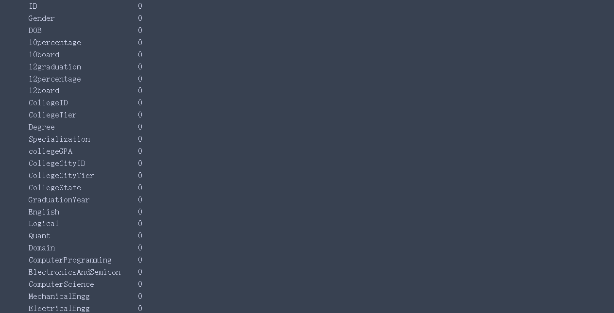
查看是否有缺失值：

data.isnull().sum()

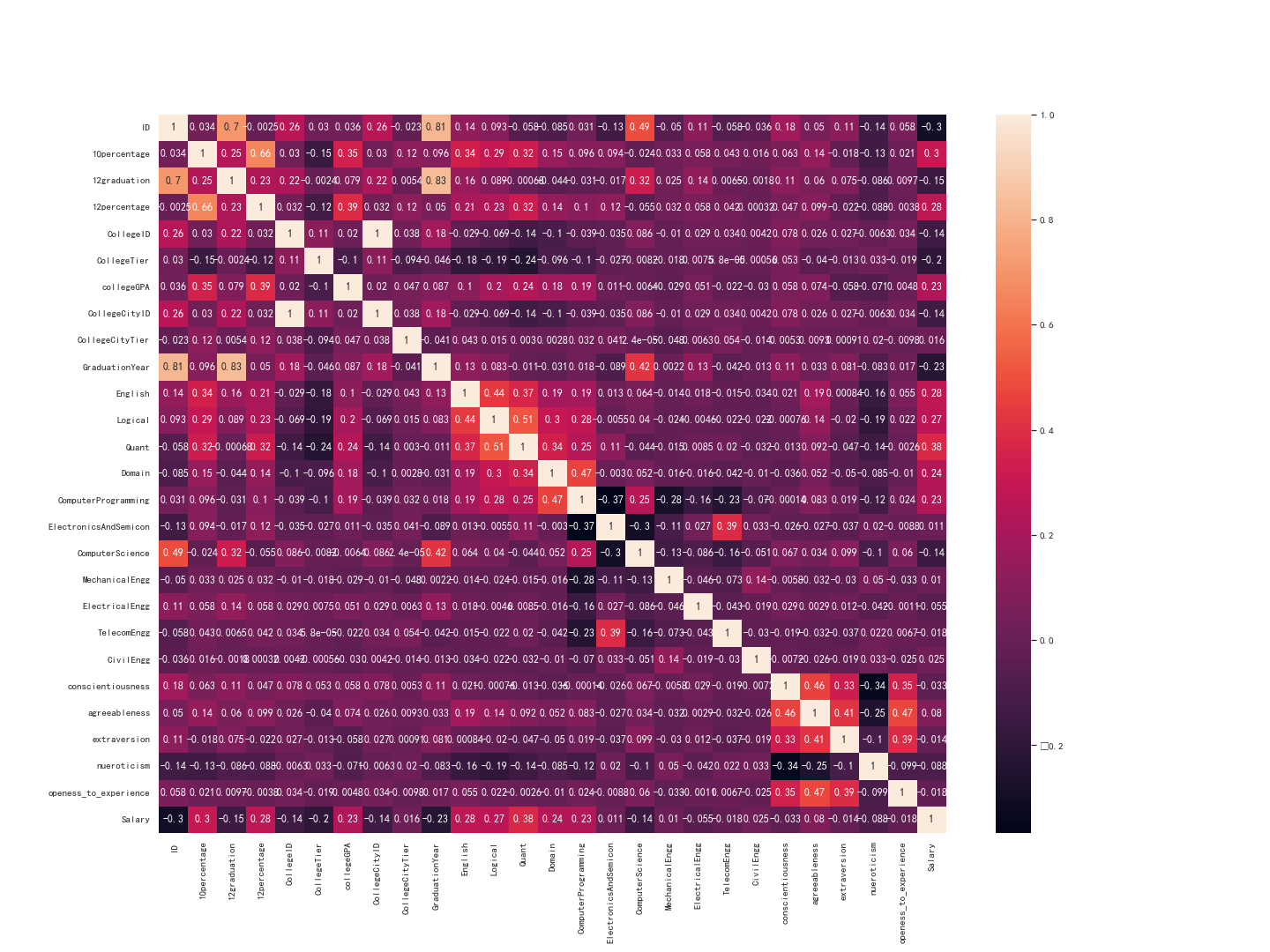
根据皮尔逊相关性绘制热力图

# seaborn中文乱码解决方案
from matplotlib.font_manager import FontProperties
myfont=FontProperties(fname=r'C:\Windows\Fonts\simhei.ttf',size=40)
sns.set(font=myfont.get_name(), color_codes=True)

data_corr = data.corr(method="spearman")#计算相关性系数
plt.figure(figsize=(20,15))#figsize可以规定热力图大小
fig=sns.heatmap(data_corr,annot=True,fmt='.2g')#annot为热力图上显示数据；fmt='.2g'为数据保留两位有效数字
fig

fig.get_figure().savefig('data_corr.png')#保留图片

下图当中，可以判断各个特征之间是否有影响，如果系数越大，则变量之间相关性越强。

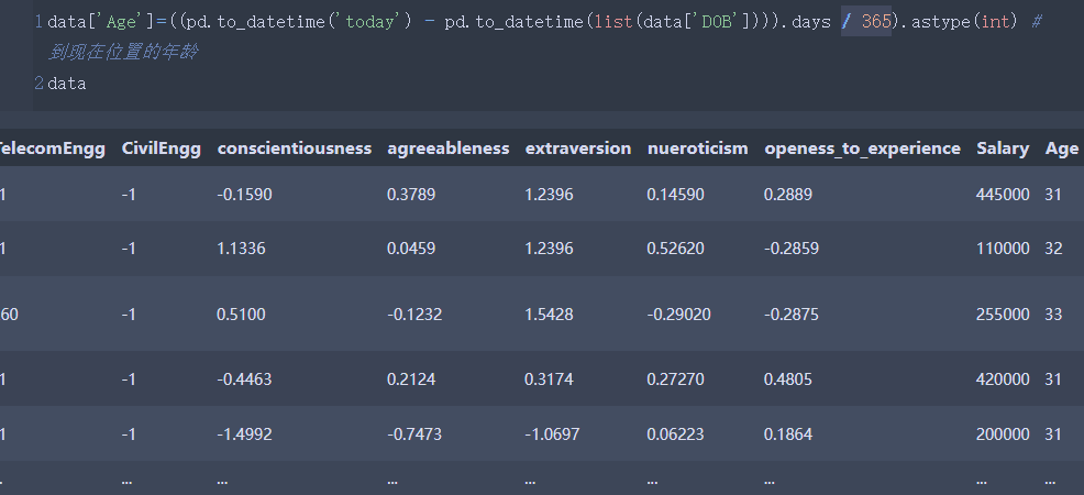
计算每个学生到现在为止的年龄：

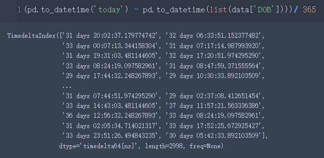
data['Age']=((pd.to_datetime('today') - pd.to_datetime(list(data['DOB']))).days / 365).astype(int) # 到现在位置的年龄
data

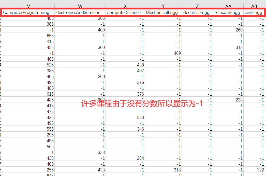
观察数据发现，在AMCAT的某些课程当中，由于许多同学没有分数，因此分数显示的是-1，所以为了进行更好的预测，在数据清理的时候将 -1 替换为总课程的平均值，以获得更好的预测。

columns = ['ComputerProgramming','ElectronicsAndSemicon','ComputerScience','MechanicalEngg','ElectricalEngg','TelecomEngg','CivilEngg']
for col in columns:
    data[col] = data[col].replace({
    
     -1 : np.nan})#先将-1填充为空值
    data[col] = data[col].fillna(data[col].mean()) #再将空值替换为平均值

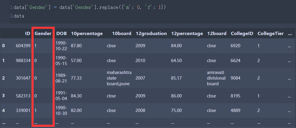
同时，将性别这列数字化：

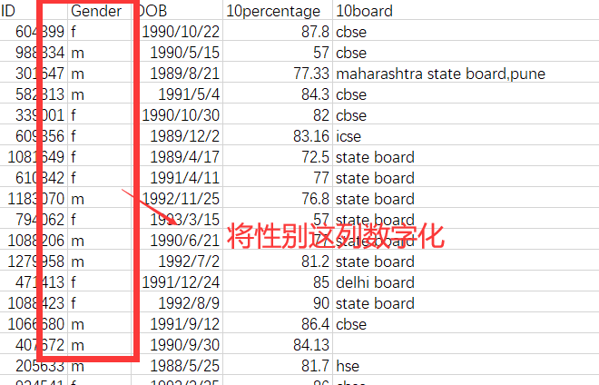
data['Gender'] = data['Gender'].replace({
    
    'm': 0, 'f': 1}) 
data

将以数字开头的属性类更改名字：

data.rename(columns ={
    
    '10percentage':'tenth_percentage','12percentage':'twelveth_percentage','10board':'tenth_board','12graduation':'twelveth_graduation','12board':'twelveth_board',}, inplace =True)
data 

data.to_csv('finish.csv')

三、第一问

分析影响高校工程类专业毕业生就业的主要因素。

根据前面的题目描述可知，我们需要使用薪水来作为就业情况的表示。

1、方法一：绘制图形

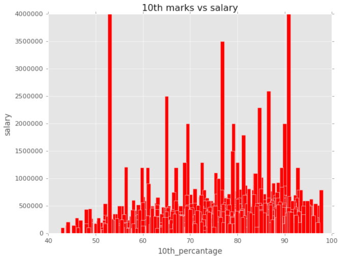
这里选择使用柱形图

plt.style.use('ggplot')
plt.bar(x.tenth_percentage,y,color ="red")
plt.xlabel("10th_percantage")#在10年级考试中获得的总成绩
plt.ylabel("salary")
plt.title("10th marks vs salary")

plt.bar(x.twelveth_percentage,y,color ="blue")
plt.xlabel("12th_percantage")#在12年级考试中获得的总成绩
plt.ylabel("salary")
plt.title("12th marks vs salary")

plt.scatter(x.CollegeTier,y,color ="pink")
plt.xlabel("CollegeTier")#学院所在城市的层
plt.ylabel("salary")
plt.title("CollegeTier vs salary")

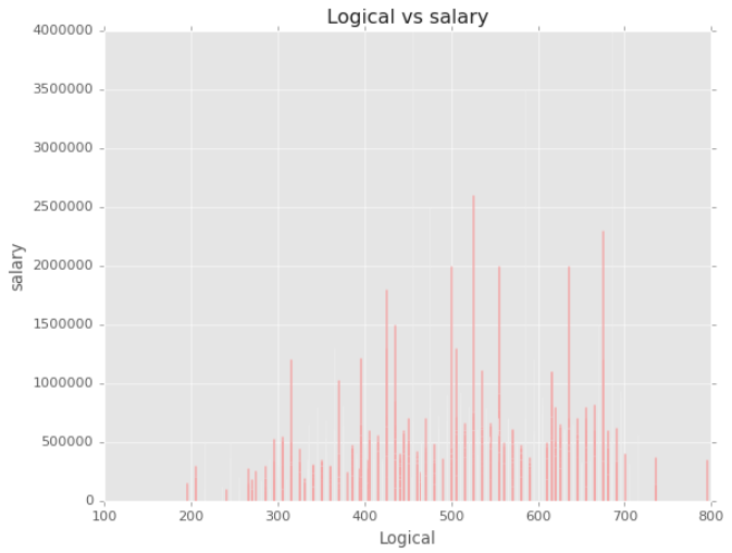
plt.bar(x.Logical,y,color ="red")
plt.xlabel("Logical")#逻辑能力
plt.ylabel("salary")
plt.title("Logical vs salary")

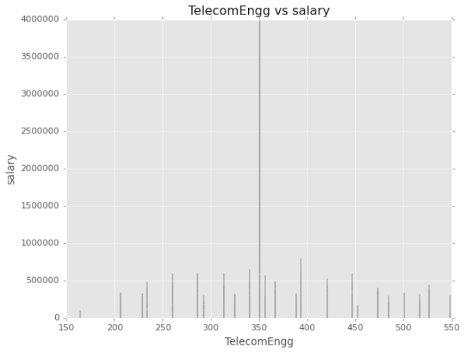
plt.bar(x.TelecomEngg,y,color ="black")
plt.xlabel("TelecomEngg")#电信工程得分
plt.ylabel("salary")
plt.title("TelecomEngg vs salary")

plt.bar(x.collegeGPA,y,color ="purple")
plt.xlabel("collegeGPA")#毕业时的GPA总计
plt.ylabel("salary")
plt.title("collegeGPA vs salary")

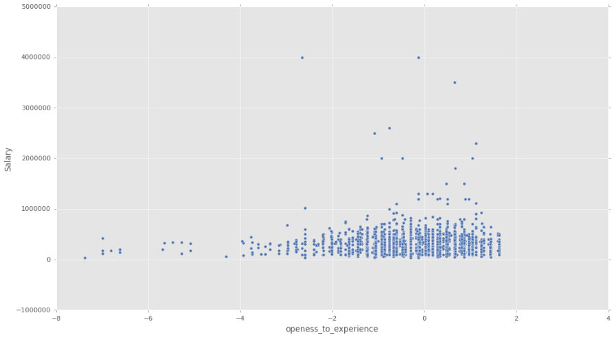
plt.figure(figsize = (15,8))
# 性格测试和薪水
sns.scatterplot(data.openess_to_experience, data.Salary, palette = 'inferno')

2、方法二：多元线性回归

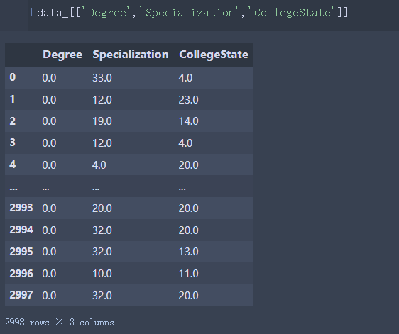
由于多元线性回归的自变量需要是数值类型，考虑把Degree，Specialization，CollegeState变成数值。

preprocessing.OrdinalEncoder：特征专用，能够将分类特征转换为分类数值

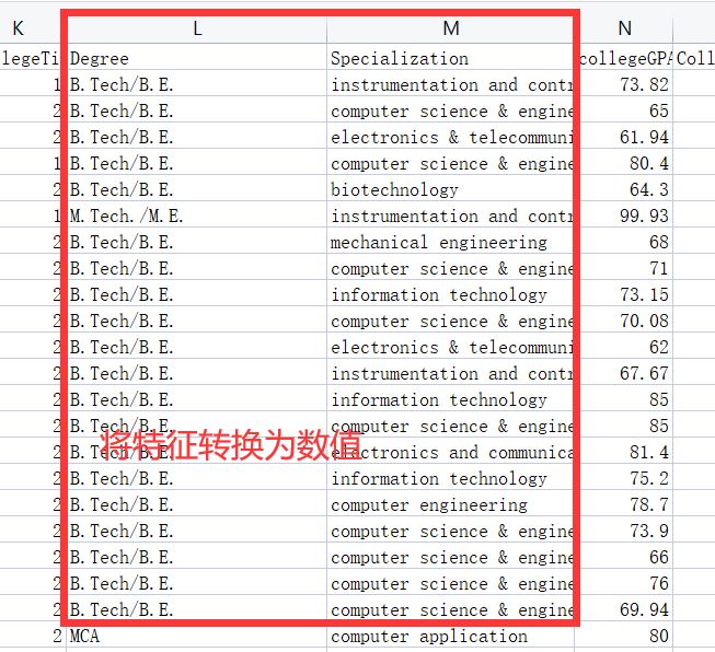
# 由于多元线性回归的自变量需要是数值类型，考虑把Degree，Specialization，CollegeState变成数值。
# preprocessing.OrdinalEncoder：特征专用，能够将分类特征转换为分类数值
from sklearn.preprocessing import OrdinalEncoder
data_=data.copy()
data_

# 取出需要转换的两个字段
OrdinalEncoder().fit(data_[['Degree','Specialization','CollegeState']]).categories_
# 使用OrdinalEncoder将字符型变成数值
data_[['Degree','Specialization','CollegeState']]=OrdinalEncoder().fit_transform(data_[['Degree','Specialization','CollegeState']])

然后我们就开始生成多元线性模型，代码如下：

x = sm.add_constant(data_[['Gender', 'tenth_percentage', 
       'twelveth_graduation', 'twelveth_percentage', 
       'CollegeID', 'CollegeTier', 'Degree', 'Specialization', 'collegeGPA',
       'CollegeCityID', 'CollegeCityTier', 'CollegeState', 'GraduationYear',
       'English', 'Logical', 'Quant', 'Domain', 'ComputerProgramming',
       'ElectronicsAndSemicon', 'ComputerScience', 'MechanicalEngg',
       'ElectricalEngg', 'TelecomEngg', 'CivilEngg', 'conscientiousness',
       'agreeableness', 'extraversion', 'nueroticism', 'openess_to_experience']]) #生成自变量
y = data['Salary'] #生成因变量
model = sm.OLS(y, x) #生成模型
result = model.fit() #模型拟合
result.summary() #模型描述

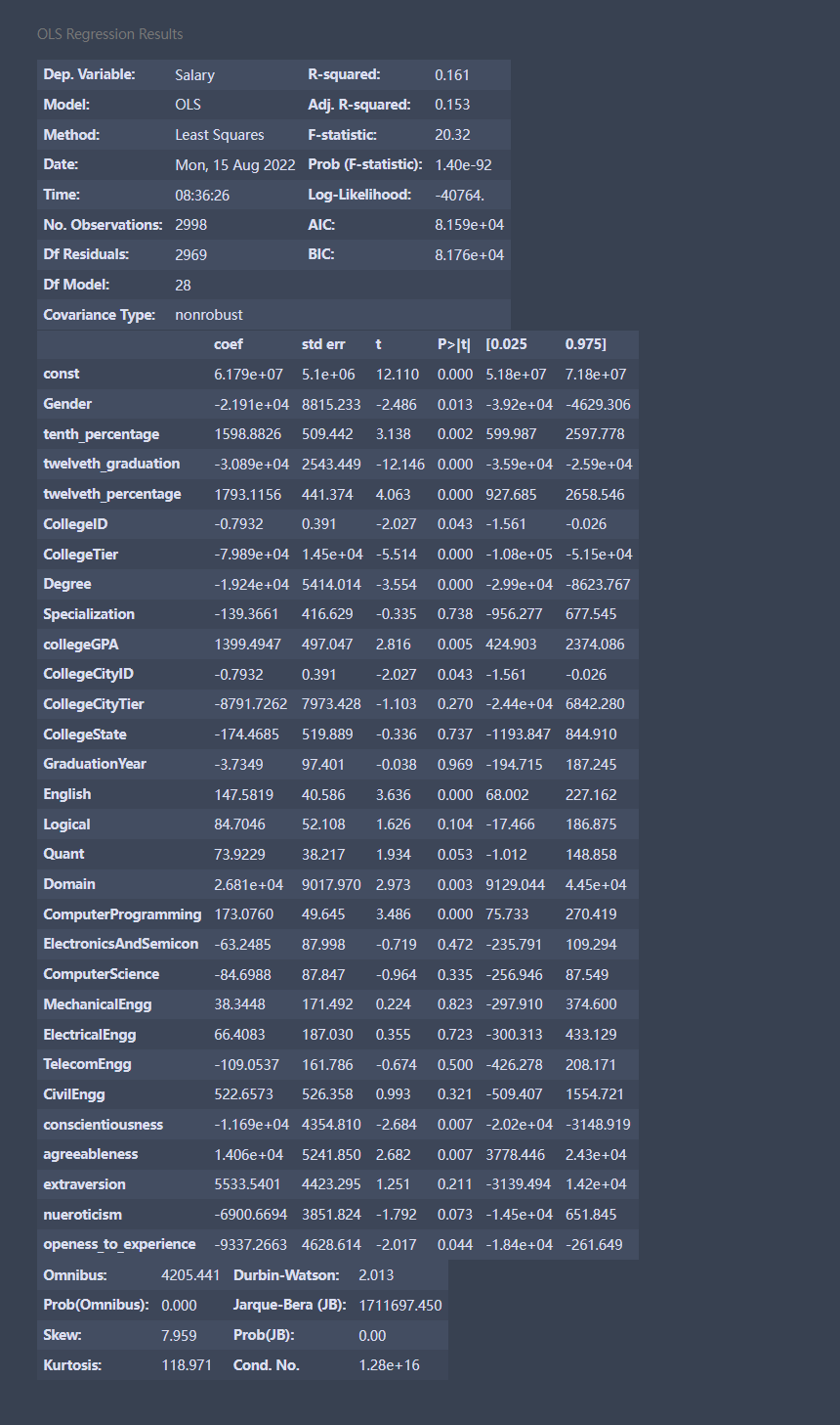
在这个结果中，我们主要看“coef”、“t”和“P>|t|”这三列。coef就是前面说过的回归系数，const这个值就是回归常数，所以我们得到的这个回归模型就是y = coef这列$\times$对应的系数。

而“t”和“P>|t|”这两列是等价的，使用时选择其中一个就行，其主要用来判断每个自变量和y的线性显著关系。从图中还可以看出，Prob (F-statistic)为1.40e-92，这个值就是我们常用的P值，其接近于零，说明我们的多元线性方程是显著的，也就是y与自变量有着显著的线性关系，而R-squared是0.161，也说明这个线性关系并不显著。

理论上，这个多元线性方程已经求出来了，但是效果一般，我们还是要进行更深一步的探讨。

前面说过，y与自变量有着显著的线性关系，这里要注意所有的自变量被看作是一个整体，y与这个整体有显著的线性关系，但不代表y与其中的每个自变量都有显著的线性关系，我们在这里要找出那些与y的线性关系不显著的自变量，然后把它们剔除，只留下关系显著的。

我们可以通过图中“P>|t|”这一列来判断，这一列中我们可以选定一个阈值，比如统计学常用的就是0.05、0.02或0.01，这里我们就用0.05，凡是P>|t|这列中数值大于0.05的自变量，我们都把它剔除掉，这些就是和y线性关系不显著的自变量，所以都舍去，请注意这里指的自变量不包括图中const这个值。

但是这里有一个原则，就是一次只能剔除一个，剔除的这个往往是P值最大的那个，比如图中P值最大的是GraduationYear，那么就把它剔除掉，然后再用剩下的自变量来重复上述建模过程，再找出P值最大的那个自变量，把它剔除，如此重复这个过程，直到所有P值都小于等于0.05，剩下的这些自变量就是我们需要的自变量，这些自变量和y的线性关系都比较显著，我们要用这些自变量来进行建模。

我们可以将上述过程写成一个函数，命名为looper，代码如下：

def looper(limit):
    cols = ['Gender', 'tenth_percentage', 
       'twelveth_graduation', 'twelveth_percentage', 
       'CollegeID', 'CollegeTier', 'Degree', 'Specialization', 'collegeGPA',
       'CollegeCityID', 'CollegeCityTier', 'CollegeState', 'GraduationYear',
       'English', 'Logical', 'Quant', 'Domain', 'ComputerProgramming',
       'ElectronicsAndSemicon', 'ComputerScience', 'MechanicalEngg',
       'ElectricalEngg', 'TelecomEngg', 'CivilEngg', 'conscientiousness',
       'agreeableness', 'extraversion', 'nueroticism', 'openess_to_experience']
    for i in range(len(cols)):
        data1 = data_[cols]
        x = sm.add_constant(data1) #生成自变量
        y = data_['Salary'] #生成因变量
        model = sm.OLS(y, x) #生成模型
        result = model.fit() #模型拟合
        pvalues = result.pvalues #得到结果中所有P值
        pvalues.drop('const',inplace=True) #把const取得
        pmax = max(pvalues) #选出最大的P值
        if pmax>limit:
            ind = pvalues.idxmax() #找出最大P值的index
            cols.remove(ind) #把这个index从cols中删除
        else:
            return result
 
result = looper(0.05)
result.summary()

由上图的相关系数可以看出，薪水和twelveth_graduation，twelveth_percentage，CollegeTier，Degree，English，ComputerProgramming具有较强的相关性。

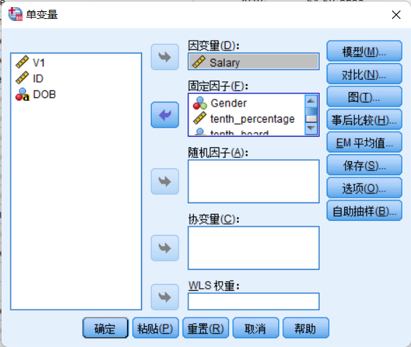
3、方法三：多因素方差分析

多因素方差分析，用于研究一个因变量是否受到多个自变量（也称为因素）的影响，它检验多个因素取值水平的不同组合之间，因变量的均值之间是否存在显著的差异。多因素方差分析既可以分析单个因素的作用（主效应），也可以分析因素之间的交互作用（交互效应），还可以进行协方差分析，以及各个因素变量与协变量的交互作用。

根据观测变量（即因变量）的数目，可以把多因素方差分析分为：单变量多因素方差分析（也叫一元多因素方差分析）与多变量多因素方差分析（即多元多因素方差分析）。本案例是一元多因素方差分析。

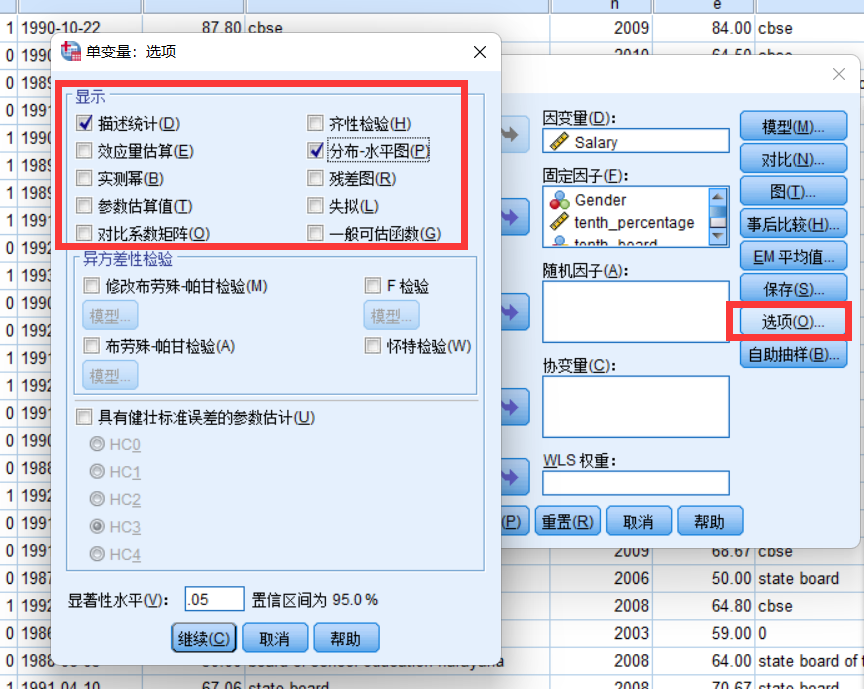
这里使用SPSS进行演示：

1、首先在文件选项卡当中导入 finish.csv 数据：

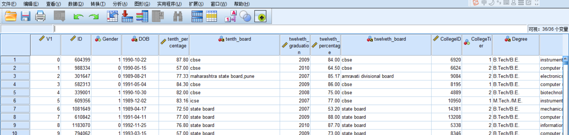
2、分析-》 一般线性模型-》单变量

4、方法四：决策树

使用机器学习算法，可以转换成决策树来得到特征重要性排名：

from sklearn import tree
# 从sklearn中导入tree

from sklearn import datasets, model_selection
# 从sklearn中导入datasets用于加载数据集，这里我们使用iris数据集
# 从sklearn中导入model_selection用户划分测试集和训练集合
feature_name = ['Gender', 'tenth_percentage', 
       'twelveth_graduation', 'twelveth_percentage', 
       'CollegeID', 'CollegeTier', 'Degree', 'Specialization', 'collegeGPA',
       'CollegeCityID', 'CollegeCityTier', 'CollegeState', 'GraduationYear',
       'English', 'Logical', 'Quant', 'Domain', 'ComputerProgramming',
       'ElectronicsAndSemicon', 'ComputerScience', 'MechanicalEngg',
       'ElectricalEngg', 'TelecomEngg', 'CivilEngg', 'conscientiousness',
       'agreeableness', 'extraversion', 'nueroticism', 'openess_to_experience','Age']
X = data_[feature_name]
Y = data_['Salary']
# 划分训练集和测试集 8:2
x_train,x_test, y_train, y_text = model_selection.train_test_split(X, Y, test_size=0.2, random_state=0)

# 创建一颗分类树，默认使用Gini
classification_tree = tree.DecisionTreeClassifier()
classification_tree.fit(x_train, y_train)
# 输出每个特征的重要性
[*zip(feature_name,classification_tree.feature_importances_)]

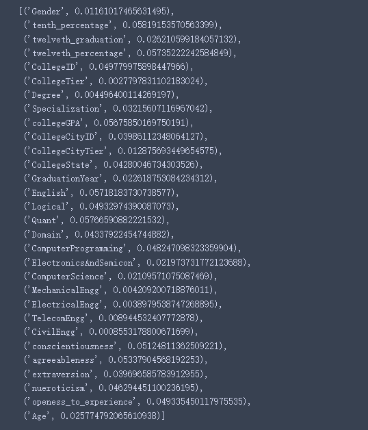
根据上面的数据就可以分析特征的重要性了。

四、第二问

根据附件一建立模型，刻画工程类专业毕业生薪水和各因素的关系。

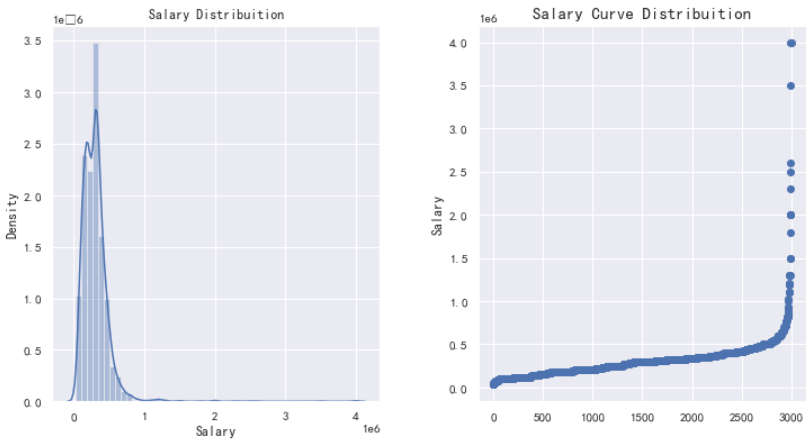
先画一下薪水分布：

plt.figure(figsize = (12, 6))

plt.subplot(121)
# 薪水分布
plt.title('Salary Distribuition')
sns.distplot(data['Salary'])

plt.subplot(122)
g1 = plt.scatter(range(data.shape[0]), np.sort(data.Salary.values))
# 薪水分布曲线
g1= plt.title("Salary Curve Distribuition", fontsize=15)
g1 = plt.xlabel("")
g1 = plt.ylabel("Salary", fontsize=12)

plt.subplots_adjust(wspace = 0.3, hspace = 0.5,
                    top = 0.9)
plt.show()

1、回归关系

这里说的是各个因素，那就要全部因素考虑进来，那就仿照第一问的方法二，可能需要把所有的object变量都变成int或者float类型，然后再进行拟合，得到具体的回归方程。

2、薪水预测

印度工科学生毕业后的工作情况和薪水。但是我们都不知道影响印度工程专业毕业生工资的不同因素是什么。该项目根据第 10 和第 12 班的分数百分比、大学等级、不同科目的分数、总体 gpa、逻辑推理和毕业年份等参数来预测工程师的薪水。该项目包括一个 ML 模型，该模型使用不同的算法来预测毕业生的薪水。这里我们使用一些主要因素来多薪水做预测（你也可以试试全部因素）。

from sklearn.preprocessing import LabelEncoder
from sklearn.preprocessing import StandardScaler
from sklearn.model_selection import train_test_split
from sklearn.linear_model import LinearRegression
from sklearn.linear_model import Ridge
from sklearn.linear_model import Lasso
from sklearn.linear_model import ElasticNet
from sklearn.neighbors import KNeighborsRegressor
from sklearn.svm import SVR, LinearSVR
from sklearn.tree import DecisionTreeRegressor
from sklearn.ensemble import RandomForestRegressor
from sklearn.ensemble import GradientBoostingRegressor
from sklearn.ensemble import AdaBoostRegressor
from sklearn.neural_network import MLPRegressor

def preprocess_inputs(data_):
    data_ = data_.copy()
    data_['Degree'] = LabelEncoder().fit_transform(data_.Degree)
    data_['Specialization'] = LabelEncoder().fit_transform(data_.Specialization)
    X=data_[['Gender', 'tenth_percentage', 
       'twelveth_graduation', 'twelveth_percentage', 
       'CollegeID', 'CollegeTier', 'Degree', 'Specialization', 'collegeGPA',
       'CollegeCityID', 'CollegeCityTier', 'CollegeState', 'GraduationYear',
       'English', 'Logical', 'Quant', 'Domain', 'ComputerProgramming',
       'ElectronicsAndSemicon', 'ComputerScience', 'MechanicalEngg',
       'ElectricalEngg', 'TelecomEngg', 'CivilEngg', 'conscientiousness',
       'agreeableness', 'extraversion', 'nueroticism', 'openess_to_experience','Age']]
    y=data_['Salary']
    X_train, X_test, y_train, y_test = train_test_split(x, y, train_size=0.7, shuffle=True, random_state=43)
    scaler = StandardScaler()
    scaler.fit(X_train)
    X_train = pd.DataFrame(scaler.transform(X_train), columns = X_train.columns, index = X_train.index)
    X_test = pd.DataFrame(scaler.transform(X_test), columns = X_test.columns, index = X_test.index)
    return X_train, X_test, y_train, y_test

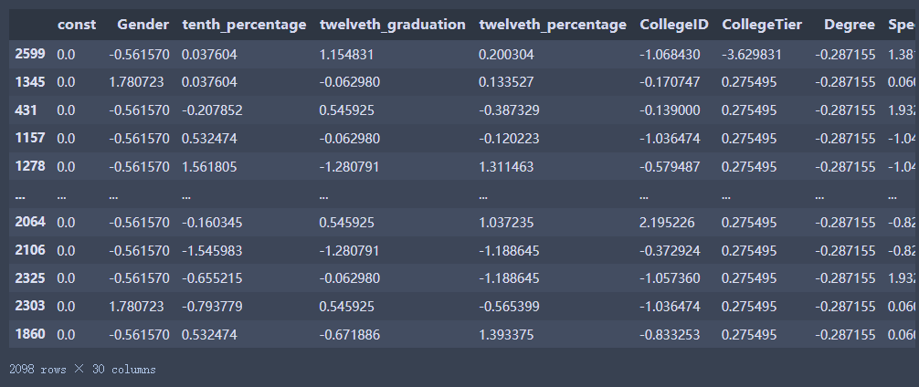
X_train, X_test, y_train, y_test = preprocess_inputs(data_)
X_train

models = {
    
    
    '  Linear Regression': LinearRegression(),
    '              Ridge': Ridge(),
    '      Decision Tree': DecisionTreeRegressor(),
    '      Random Forest': RandomForestRegressor(random_state=100,
                             bootstrap=True,
                            max_depth=2,
                             max_features=2,
                            min_samples_leaf=3,
                            min_samples_split=5,
                            n_estimators=3),
    '             Lasso' : Lasso(),
    '       Elastic Net' : ElasticNet(),
    '    Neural network' : MLPRegressor(),
    '  Gradient Boosting': GradientBoostingRegressor(),
    'Adaboost Classifier': AdaBoostRegressor(),
    'KNN': KNeighborsRegressor()
}

for name, model in models.items():
    model = model.fit(X_train, y_train)
    print(name + " trained")

for name, model in models.items():
    print(name,model.score(X_test, y_test))

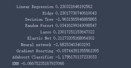
emmmmmm，训练的结果最好的也才0.23，不是很理想

五、第三问

根据以上的分析，对我国高校工程类专业学生培养是否有一定的启迪？写一份建议书。

注意不要乱写，不是让你编个小论文，要根据前面两个问题进行分析，从而写关于我国的建议（注意：针对自己本校就行了）。最终目的是希望学生的就业薪水更高。

比如哪些因素不应该过度严厉，哪些因素学校应该严抓等。。。。应该有这方面论文,去找找。

参考：

1、对学校就业工作的建议

2、大学生就业形势

3、对学校人才培养工作有何建议