机器学习笔记 - 构建推荐系统(4) 用于协同过滤的矩阵分解

一、协同过滤概述

        协同过滤是任何现代推荐系统的核心，它在亚马逊、Netflix 和 Spotify 等公司取得了相当大的成功。它的工作原理是收集给定域中项目的人类判断（称为评级），并将具有相同信息需求或相同品味的人匹配在一起。协同过滤系统的用户分享他们对他们消费的每个项目的分析判断和意见，以便系统的其他用户可以更好地决定消费哪些项目。作为回报，协同过滤系统为新项目提供有用的个性化推荐。

        协同过滤的两个主要领域是（1）邻域方法和（2）潜在因子模型。

• 邻域方法专注于计算项目之间或用户之间的关系。这种方法基于同一用户对相邻项目的评分来评估用户对项目的偏好。一个项目的邻居是其他产品，当由同一用户评分时，它们往往会获得相似的评分。
• 潜在因素方法通过从评分模式推断出的许多因素对项目和用户进行表征来解释评分。例如，在音乐推荐中，发现的因素可能会测量精确的维度，例如嘻哈与爵士乐、高音的数量或歌曲的长度，以及不太明确的维度，例如歌词背后的含义，或完全无法解释的尺寸。对于用户，每个因素衡量用户喜欢在相应歌曲因素上得分高的歌曲的程度。

        一些最成功的潜在因子模型是基于矩阵分解的。在其自然形式中，矩阵分解使用从项目评级模式推断的因素向量来表征项目和用户。项目和用户因素之间的高度对应导致推荐。

二、Vanilla Matrix Factorization

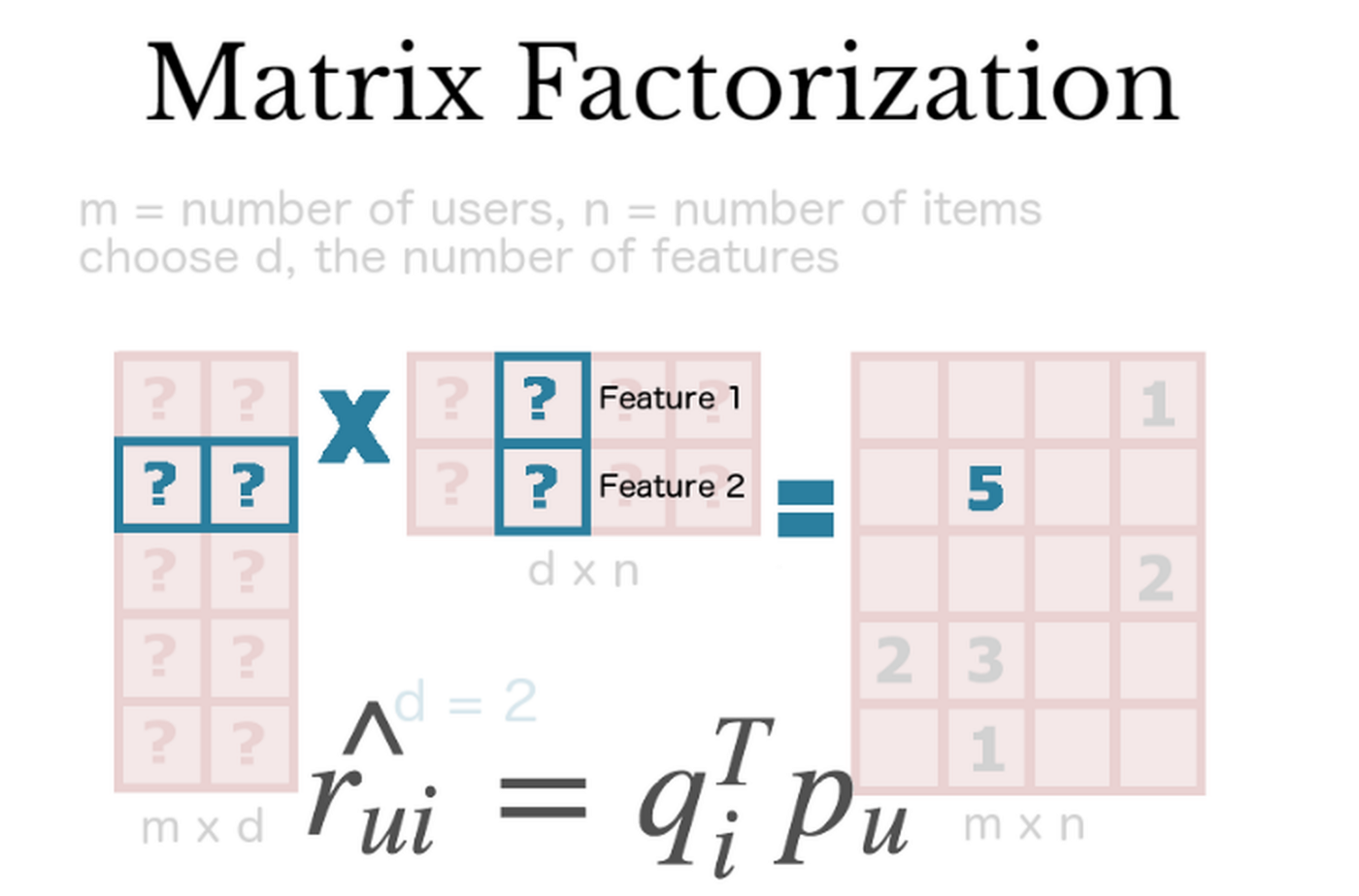
        一个简单的矩阵分解模型将用户和项目都映射到维数为 D 的联合潜在因子空间—这样用户-项目的交互就被建模为该空间中的内积。

• 因此，每个项目 i 与向量 q_i 相关联，并且每个用户 u 与向量 p_u 相关联。
• 对于给定的项目 i，q_i 的元素衡量项目拥有这些因素的程度，无论是积极的还是消极的。
• 对于给定的用户 u，p_u 的元素衡量用户对相应因素（正面或负面）高的项目的兴趣程度。
• 得到的点积 (q_i * p_u) 捕获了用户 u 和项目 i 之间的交互，即用户对项目特征的整体兴趣。

        因此，我们有如下等式1：

        最大的挑战是计算每个项目和用户到因子向量 q_i 和 p_u 的映射。矩阵分解通过最小化已知评级集上的正则化平方误差来做到这一点，如下面的等式 2 所示：

        该模型是通过拟合先前观察到的评级来学习的。然而，目标是以预测未来/未知评级的方式概括这些先前的评级。因此，我们希望通过向每个元素添加 L2 正则化惩罚来避免过度拟合观察到的数据，并与随机梯度下降同时优化学习参数。

        当我们使用 SGD 将模型的参数拟合到手头的学习问题时，我们在解决方案空间中朝着损失函数在算法每次迭代中相对于网络参数的梯度迈出了一步。由于我们推荐中的用户-项目交互矩阵非常稀疏，这种学习方法可能会过度拟合训练数据。

        L2是一种通过添加复杂性表示项来正则化成本函数的特定方法。该术语是用户和项目潜在因素的平方欧几里得范数。添加了一个附加参数 λ 以允许控制正则化的强度。添加 L2 项通常会导致整个模型的参数更小。

import torch
from torch import nn
import torch.nn.functional as F

class MF(nn.Module):
  
  def __call__(self, train_x):

        # These are the user indices, and correspond to "u" variable
        user_id = train_x[:, 0]
        # These are the item indices, correspond to the "i" variable
        item_id = train_x[:, 1]

        # Initialize a vector user = p_u using the user indices
        vector_user = self.user(user_id)
        # Initialize a vector item = q_i using the item indices
        vector_item = self.item(item_id)

        # The user-item interaction: p_u * q_i is a dot product between the 2 vectors above
        ui_interaction = torch.sum(vector_user * vector_item, dim=1)
        
        return ui_interaction

    def loss(self, prediction, target):

        # Calculate the Mean Squared Error between target = R_ui and prediction = p_u * q_i
        loss_mse = F.mse_loss(prediction, target.squeeze())

        # Compute L2 regularization over user (P) and item (Q) matrices
        prior_user = l2_regularize(self.user.weight) * self.c_vector
        prior_item = l2_regularize(self.item.weight) * self.c_vector

        # Add up the MSE loss + user & item regularization
        total = loss_mse + prior_user + prior_item
        
        return total

三、带偏差的矩阵分解

        协同过滤的矩阵分解方法的一个好处是它在处理各种数据方面和其他特定于应用程序的要求方面的灵活性。回想一下，等式 1 试图捕捉用户和产生不同评分值的项目之间的交互。然而，观察到的评分值的大部分变化是由于与用户或项目相关的影响，称为偏差，与任何交互无关。这背后的直觉是，一些用户给予的评价比其他用户高，而一些项目系统地获得了比其他用户高的评价。

因此，我们可以将等式 1 扩展到等式 3，如下所示：

• 总体平均评分中涉及的偏差用 b 表示。
• 参数 w_i 和 w_u 分别表示观察到的项目 i 和用户 u 与平均值的偏差。
• 请注意，观察到的评分分为 4 个部分：（1）用户-项目交互，（2）全局平均值，（3）项目偏差和（4）用户偏差。

        该模型是通过最小化一个新的平方误差函数来学习的，如下面的等式 4 所示：

import torch
from torch import nn
import torch.nn.functional as F

class MF(nn.Module):
  
  def __call__(self, train_x):

        # These are the user indices, and correspond to "u" variable
        user_id = train_x[:, 0]
        # These are the item indices, correspond to the "i" variable
        item_id = train_x[:, 1]

        # Initialize a vector user = p_u using the user indices
        vector_user = self.user(user_id)
        # Initialize a vector item = q_i using the item indices
        vector_item = self.item(item_id)

        # The user-item interaction: p_u * q_i is a dot product between the 2 vectors above
        ui_interaction = torch.sum(vector_user * vector_item, dim=1)

        # Pull out biases
        bias_user = self.bias_user(user_id).squeeze()
        bias_item = self.bias_item(item_id).squeeze()
        biases = (self.bias + bias_user + bias_item)

        # Add the bias to the user-item interaction to obtain the final prediction
        prediction = ui_interaction + biases
        
        return prediction

    def loss(self, prediction, target):

        # Calculate the Mean Squared Error between target and prediction
        loss_mse = F.mse_loss(prediction, target.squeeze())

        # Compute L2 regularization over the biases for user and the biases for item matrices
        prior_bias_user = l2_regularize(self.bias_user.weight) * self.c_bias
        prior_bias_item = l2_regularize(self.bias_item.weight) * self.c_bias

        # Compute L2 regularization over user (P) and item (Q) matrices
        prior_user = l2_regularize(self.user.weight) * self.c_vector
        prior_item = l2_regularize(self.item.weight) * self.c_vector

        # Add up the MSE loss + user & item regularization + user & item biases regularization
        total = loss_mse + prior_user + prior_item + prior_bias_user + prior_bias_item

        return total

四、具有边特征的矩阵分解

        协同过滤的一个常见挑战是冷启动问题，因为它无法处理新项目和新用户。或者许多用户提供的评分很少，使得用户-项目交互矩阵非常稀疏。缓解此问题的一种方法是合并有关用户的其他信息源，即附加功能。这些可以用户属性（人口统计）和隐式反馈.

        回到例子，假设我知道用户的职业。对于这个附加功能，有两个选择：将其添加为偏见（艺术家比其他职业更喜欢电影）并将其添加为向量（房地产经纪人喜欢房地产节目）。矩阵分解模型应将所有信号源与增强的用户表示相结合，如等式 5 所示：

• 职业的偏差用 d_o 表示，这意味着职业的变化与比率一样。
• 职业的向量用 t_o 表示，这意味着职业会根据项目（q_i * t_o）而变化。
• 请注意，物品在必要时可以得到类似的处理。

        损失函数现在看起来如何？下面的公式 6 表明：

import torch
from torch import nn
import torch.nn.functional as F

class MF(nn.Module):
  
  def __call__(self, train_x):

        # These are the user indices, and correspond to "u" variable
        user_id = train_x[:, 0]
        # These are the item indices, correspond to the "i" variable
        item_id = train_x[:, 1]

        # Initialize a vector user = p_u using the user indices
        vector_user = self.user(user_id)
        # Initialize a vector item = q_i using the item indices
        vector_item = self.item(item_id)

        # The user-item interaction: p_u * q_i is a dot product between the user vector and the item vector
        ui_interaction = torch.sum(vector_user * vector_item, dim=1)

        # Pull out biases
        bias_user = self.bias_user(user_id).squeeze()
        bias_item = self.bias_item(item_id).squeeze()
        biases = (self.bias + bias_user + bias_item)

        # These are the occupation indices, and correspond to "o" variable
        occu_id = train_x[:, 3]
        # Initialize a vector occupation = r_o using the occupation indices
        vector_occu = self.occu(occu_id)
        # The user-occupation interaction: p_u * r_o is a dot product between the user vector and the occupation vector
        uo_interaction = torch.sum(vector_user * vector_occu, dim=1)

        # Add the bias, the user-item interaction, and the user-occupation interaction to obtain the final prediction
        prediction = ui_interaction + uo_interaction + biases
        
        return prediction
      
  def loss(self, prediction, target):

        # Calculate the Mean Squared Error between target and prediction
        loss_mse = F.mse_loss(prediction.squeeze(), target.squeeze())

        # Compute L2 regularization over the biases for user and the biases for item matrices
        prior_bias_user = l2_regularize(self.bias_user.weight) * self.c_bias
        prior_bias_item = l2_regularize(self.bias_item.weight) * self.c_bias

        # Compute L2 regularization over user (P) and item (Q) matrices
        prior_user = l2_regularize(self.user.weight) * self.c_vector
        prior_item = l2_regularize(self.item.weight) * self.c_vector

        # Compute L2 regularization over occupation (R) matrices
        prior_occu = l2_regularize(self.occu.weight) * self.c_vector

        # Add up the MSE loss + user & item regularization + user & item biases regularization + occupation regularization
        total = loss_mse + prior_user + prior_item + prior_bias_item + prior_bias_user + prior_occu

        return total

五、具有时间特征的矩阵分解

        到目前为止，我们的矩阵分解模型一直是静态的。在现实中，物品流行度和用户偏好不断变化。因此，我们应该考虑反映用户-项目交互动态性质的时间效应。为了实现这一点，我们可以添加一个影响用户偏好的时间项，从而影响用户和项目之间的交互。

        为了稍微混合一下，让我们尝试下面的新公式 7，其中包含时间 t 评级的动态预测规则：

• 将用户因素作为时间的函数。另一方面，保持不变，因为项目是静态的。
• 我们根据用户（）进行职业更改。

        等式 8 显示了包含时间特征的新损失函数：

import torch
from torch import nn
import torch.nn.functional as F

class MF(nn.Module):
  
  def __call__(self, train_x):

        # These are the user indices, and correspond to "u" variable
        user_id = train_x[:, 0]
        # These are the item indices, correspond to the "i" variable
        item_id = train_x[:, 1]
        # These are the occupation indices, and correspond to "o" variable
        occu_id = train_x[:, 3]

        # Initialize a vector user = p_u using the user indices
        vector_user = self.user(user_id)
        # Initialize a vector item = q_i using the item indices
        vector_item = self.item(item_id)
        # Initialize a vector occupation = r_o using the occupation indices
        vector_occu = self.occu(occu_id)

        # Pull out biases
        bias_user = self.bias_user(user_id).squeeze()
        bias_item = self.bias_item(item_id).squeeze()
        biases = (self.bias + bias_user + bias_item)

        # The user-item interaction: p_u * q_i is a dot product between the user vector and the item vector
        ui_interaction = torch.sum(vector_user * vector_item, dim=1)
        # The user-occupation interaction: p_u * r_o is a dot product between the user vector and the occupation vector
        uo_interaction = torch.sum(vector_user * vector_occu, dim=1)

        # These are the rank indices
        rank = train_x[:, 2]
        # Initialize a vector temporal using the rank indices
        vector_temp = self.temp(rank)
        # Initialize a vector user-temporal using the user IDs
        vector_user_temp = self.user_temp(user_id)
        # The user-time interaction is a dot product between the user temporal vector and the temporal vector
        ut_interaction = torch.sum(vector_user_temp * vector_temp, dim=1)

        # Final prediction is the sum of all these interactions with the biases
        prediction = ui_interaction + uo_interaction + ut_interaction + biases
        
        return prediction

    def loss(self, prediction, target):

        # Calculate the Mean Squared Error between target and prediction
        loss_mse = F.mse_loss(prediction.squeeze(), target.squeeze())

        # Compute L2 regularization over the biases for user and the biases for item matrices
        prior_bias_user = l2_regularize(self.bias_user.weight) * self.c_bias
        prior_bias_item = l2_regularize(self.bias_item.weight) * self.c_bias

        # Compute L2 regularization over user (P), item (Q), and occupation (R) matrices
        prior_user = l2_regularize(self.user.weight) * self.c_vector
        prior_item = l2_regularize(self.item.weight) * self.c_vector
        prior_occu = l2_regularize(self.occu.weight) * self.c_vector

        # Compute L2 regularization over temporal matrices
        prior_ut = l2_regularize(self.user_temp.weight) * self.c_ut
        # Compute total variation regularization over temporal matrices
        prior_tv = total_variation(self.temp.weight) * self.c_temp

        # Add up the MSE loss + user & item & occupation regularization + user & item biases regularization +
        # temporal regularization + total variation
        total = loss_mse + prior_user + prior_item + prior_ut + \
                prior_bias_item + prior_bias_user + prior_occu + prior_tv

        return total

六、分解机

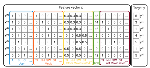
        推荐系统中一种更强大的技术称为分解机，它具有强大的、表达能力来概括矩阵分解方法。在许多应用程序中，我们有大量的项目元数据可用于做出更好的预测。这是将因子分解机与特征丰富的数据集一起使用的好处之一，其中有一种自然的方式可以在模型中包含额外的特征，并且可以使用维度参数 d 对高阶交互进行建模。对于稀疏数据集，二阶分解机模型就足够了，因为没有足够的信息来估计更复杂的交互。

        Berwyn Zhang — 分解机 ( http://berwynzhang.com/2017/01/22/machine_learning/Factorization_Machines/ )

        等式 9 显示了二阶 FM 模型的样子：

        其中 v 表示与每个变量（用户和项目）相关的 k 维潜在向量，括号运算符表示内积。根据 Steffen Rendle关于因子分解机的原始论文，如果我们假设每个 x(j) 向量仅在位置 u 和 i 处非零，我们将得到经典的带有偏差的矩阵分解模型（等式 3）：

        这两个方程之间的主要区别在于，因子分解机在潜在向量方面引入了高阶交互，这些潜在向量也受分类或标签数据的影响。这意味着模型超越了共现，以找到每个特征的潜在表示之间更强的关系。

        Factorization Machines 模型的损失函数只是均方误差和特征集的总和，如等式 10 所示：

import torch
from torch import nn
import torch.nn.functional as F

class MF(nn.Module):
  
  def __call__(self, train_x):

        # Pull out biases
        biases = index_into(self.bias_feat.weight, train_x).squeeze().sum(dim=1)

        # Initialize vector features using the feature weights
        vector_features = index_into(self.feat.weight, train_x)

        # Use factorization machines to pull out the interactions
        interactions = factorization_machine(vector_features).squeeze().sum(dim=1)

        # Final prediction is the sum of biases and interactions
        prediction = biases + interactions
        
        return prediction

    def loss(self, prediction, target):

        # Calculate the Mean Squared Error between target and prediction
        loss_mse = F.mse_loss(prediction.squeeze(), target.squeeze())

        # Compute L2 regularization over feature matrices
        prior_feat = l2_regularize(self.feat.weight) * self.c_feat

        # Add the MSE loss and feature regularization to get total loss
        total = (loss_mse + prior_feat)

        return total

七、混合口味的矩阵分解

        迄今为止提出的技术隐含地将用户品味视为单峰——也就是在单个潜在向量中。这可能会导致在代表用户时缺乏细微差别，在这种情况下，主导品味可能会压倒更多利基品味。此外，这可能会降低项目表示的质量，从而减少属于多种品味/类型的项目组之间嵌入空间的分离。

Maciej KulaMaciej Kula提出并评估将用户表示为混合物，如果有几种不同的口味，由不同的口味向量表示。每个味觉向量都与一个注意力向量相结合，描述了它在评估任何给定项目时的能力。然后将用户的偏好建模为所有用户口味的加权平均值，权重由每种口味与评估给定项目的相关程度提供。

        等式 11 给出了这个混合口味模型的数学公式：

• 是代表用户 u 的 m 种口味的 amxk 矩阵。
• 是 amxk 矩阵，表示来自 U_u 的每种口味的亲和力，用于表示特定项目。
• 是 soft-max 激活函数。
• 给出混合概率。
• 给出每个混合成分的推荐分数。
• 请注意，我们假设所有混合成分的恒等方差矩阵。

        因此，下面的等式 12 捕获了损失函数：

import torch
from torch import nn
import torch.nn.functional as F

class MF(nn.Module):
  
  def __call__(self, train_x):

        # These are the user and item indices
        user_id = train_x[:, 0]
        item_id = train_x[:, 1]

        # Initialize a vector item using the item indices
        vector_item = self.item(item_id)

        # Pull out biases
        bias_user = self.bias_user(user_id).squeeze()
        bias_item = self.bias_item(item_id).squeeze()
        biases = (self.bias + bias_user + bias_item)

        # **NEW: Initialize the user taste & attention matrices using the user IDs
        user_taste = self.user_taste[user_id]
        user_attention = self.user_attention[user_id]

        vector_itemx = vector_item.unsqueeze(2).expand_as(user_attention)
        attention = F.softmax(user_attention * vector_itemx, dim=1)
        attentionx = attention.sum(2).unsqueeze(2).expand_as(user_attention)

        # Calculate the weighted preference to be the dot product of the user taste and attention
        weighted_preference = (user_taste * attentionx).sum(2)
        # This is a dot product of the weighted preference and vector item
        dot = (weighted_preference * vector_item).sum(1)

        # Final prediction is the sum of the biases and the dot product above
        prediction = dot + biases
        
        return prediction

    def loss(self, prediction, target):

        # Calculate the Mean Squared Error between target and prediction
        loss_mse = F.mse_loss(prediction.squeeze(), target.squeeze())

        # Compute L2 regularization over the biases for user and the biases for item matrices
        prior_bias_user = l2_regularize(self.bias_user.weight) * self.c_bias
        prior_bias_item = l2_regularize(self.bias_item.weight) * self.c_bias

        # Compute L2 regularization over the user tastes and user attentions matrix
        prior_taste = l2_regularize(self.user_taste) * self.c_vector
        prior_attention = l2_regularize(self.user_attention) * self.c_vector

        # Compute L2 regularization over item matrix
        prior_item = l2_regularize(self.item.weight) * self.c_vector

        # Add up the MSE loss + user & item biases regularization + item regularization + user taste & attention regularization
        total = (loss_mse + prior_bias_item + prior_bias_user + prior_taste + prior_attention + prior_item)

        return total

八、变分矩阵分解

        我要介绍的最后一个矩阵分解变体称为变分矩阵分解。虽然到目前为止博客文章讨论的大部分内容都是关于优化模型参数的点估计，但变分是关于优化后验，粗略地说，它表达了与数据一致的一系列模型配置。

        以下是变分的实际原因：

• 变分方法可以提供替代的正则化。
• 变分方法可以测量您的模型不知道的内容。
• 变分方法可以揭示蕴涵以及对数据进行分组的新颖方法。

        我们可以通过以下方式使方程 3 中的矩阵分解变分：（1）用分布中的样本替换点估计，以及（2）用正则化新分布替换正则化该点。数学相当复杂。关于变分贝叶斯方法的维基百科页面是一个入门指南。最常见的变分贝叶斯类型使用Kullback-Leibler 散度作为不相似函数的选择，这使得损失最小化易于处理。

import torch
from torch import nn
import torch.nn.functional as F

class MF(nn.Module):
  
  def __call__(self, train_x):

        # These are the user and item indices
        user_id = train_x[:, 0]
        item_id = train_x[:, 1]

        # *NEW: Stochastically-sampled user & item vectors
        vector_user = sample_gaussian(self.user_mu(user_id), self.user_lv(user_id))
        vector_item = sample_gaussian(self.item_mu(item_id), self.item_lv(item_id))

        # Pull out biases
        bias_user = self.bias_user(user_id).squeeze()
        bias_item = self.bias_item(item_id).squeeze()
        biases = (self.bias + bias_user + bias_item)

        # The user-item interaction is a dot product between the user and item vectors
        ui_interaction = torch.sum(vector_user * vector_item, dim=1)

        # Final prediction is the sum of the user-item interaction with the biases
        prediction = ui_interaction + biases
        
        return prediction

    def loss(self, prediction, target):

        # Calculate the Mean Squared Error between target and prediction
        loss_mse = F.mse_loss(prediction.squeeze(), target.squeeze())

        # Compute L2 regularization over the biases for user and the biases for item matrices
        prior_bias_user = l2_regularize(self.bias_user.weight) * self.c_bias
        prior_bias_item = l2_regularize(self.bias_item.weight) * self.c_bias

        # *NEW: Compute the KL-Divergence loss over the Mu and Log-Variance for user and item matrices
        user_kld = gaussian_kldiv(self.user_mu.weight, self.user_lv.weight) * self.c_kld
        item_kld = gaussian_kldiv(self.item_mu.weight, self.item_lv.weight) * self.c_kld

        # Add up the MSE loss + user & item biases regularization + user & item KL-Divergence loss
        total = loss_mse + prior_bias_user + prior_bias_item + user_kld + item_kld

        return total

九、总结

        完整代码参考

MetaRec/Matrix-Factorization-Experiments at master · khanhnamle1994/MetaRec · GitHubPyTorch Implementations For A Series Of Deep Learning-Based Recommendation Models (IN PROGRESS) - MetaRec/Matrix-Factorization-Experiments at master · khanhnamle1994/MetaRechttps://github.com/khanhnamle1994/MetaRec/tree/master/Matrix-Factorization-Experiments        模型评估结果

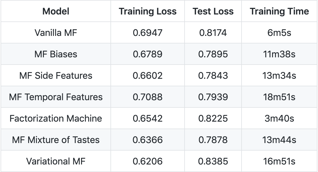
• 变分矩阵分解具有最低的训练损失。
• 具有边特征的矩阵分解具有最低的测试损失。
• Factorization Machines 的训练时间最快。