1. 背景介绍
2. 数据准备
打开excel,数据集如下,其实我们只要开始价格open,最高价(High),最低价(low)这三列。

3. 理论讲解
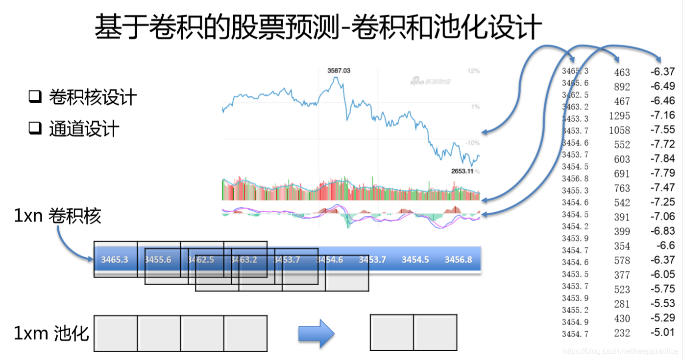
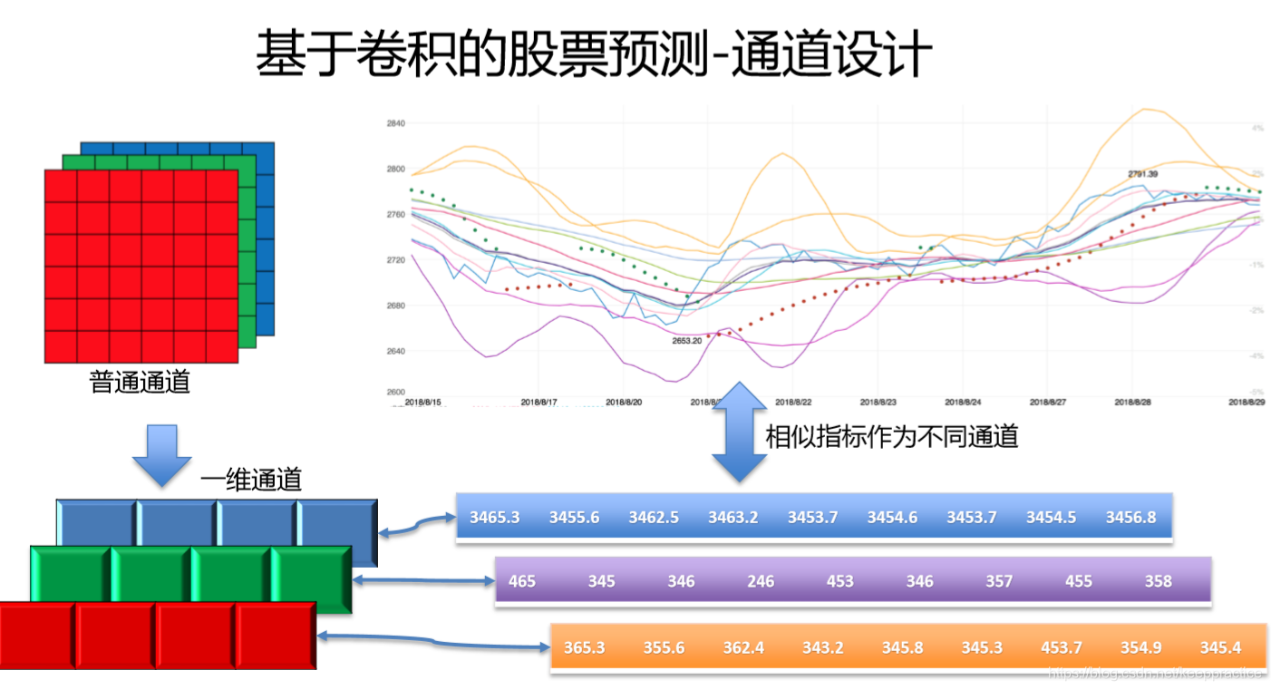
提取数据集的open, high, low这三列。利用窗口大小为90,每90行最为一个整体并且根据这90行的Label选出最多的值最为最终的Label值,数据集的shape是(141, 90, 3)
4. 代码讲解
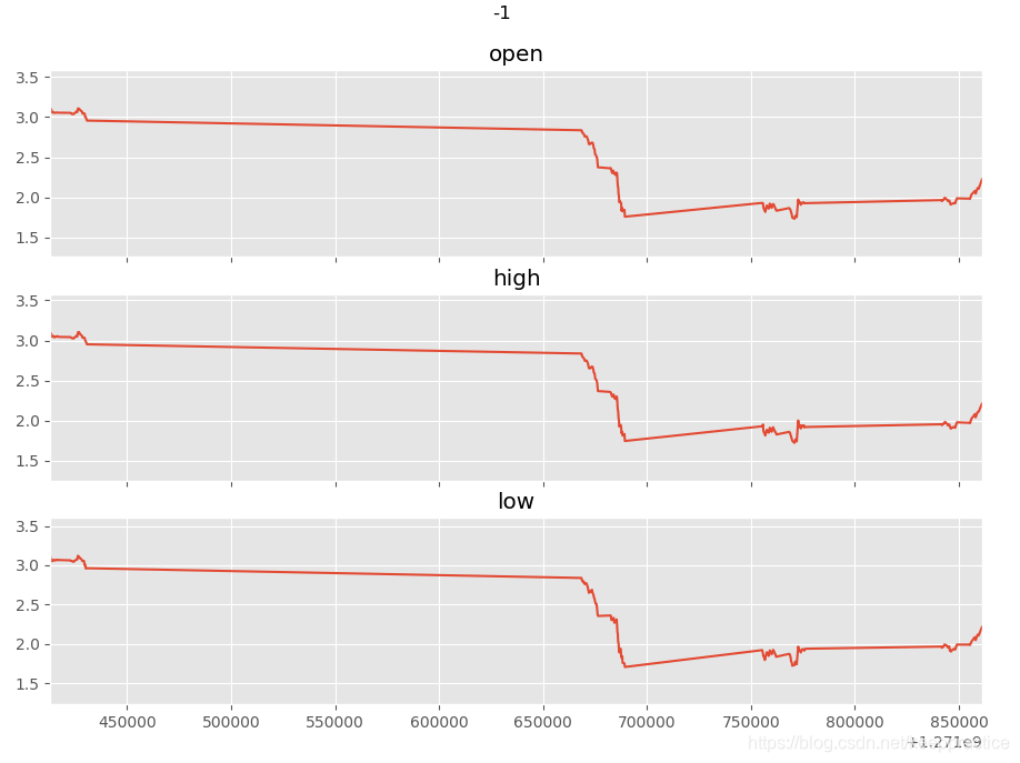
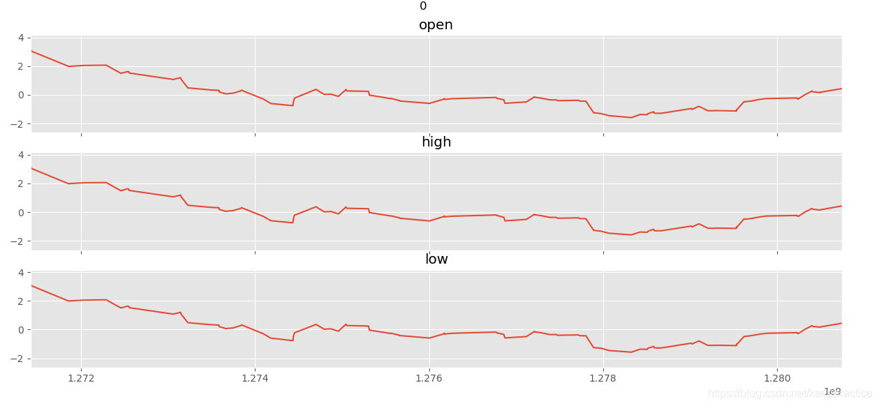
提取数据集的open, high, low这三列。标准化每一列的值。然后利用窗口大小为90,每90行最为一个整体并且根据这90行的Label选出最多的值最为最终的Label值,数据集的shape是(141, 90, 3)
最后利用matplotlib 把数据显示出来。
import pandas as pd
import numpy as np
import matplotlib.pyplot as plt
from scipy import stats
import tensorflow.compat.v1 as tf
tf.disable_v2_behavior()

import os
import warnings


#%matplotlib inline
os.environ['TF_CPP_MIN_LOG_LEVEL'] = '3' #Hide messy TensorFlow warnings
warnings.filterwarnings("ignore") #Hide messy Numpy warnings

plt.style.use('ggplot')

def read_data(file_path):
    file=pd.read_csv(file_path)
    data=file[['timestamp','open','high','low','close','vol','holdingvol','ZTM:MACD','ZTM:RSI','ZTM:ma5','ZTM:ma7','ZTM:ma10','ZTM:ma21','label']]

    return data

def feature_normalize(dataset):
    mu = np.mean(dataset,axis = 0)
    sigma = np.std(dataset,axis = 0)
    return (dataset - mu)/sigma

def plot_axis(ax, x, y, title):
    ax.plot(x, y)
    ax.set_title(title)
    ax.xaxis.set_visible(False)
    ax.set_ylim([min(y) - np.std(y), max(y) + np.std(y)])
    ax.set_xlim([min(x), max(x)])
    ax.grid(True)

def plot_activity(activity,data):
    fig, (ax0, ax1, ax2) = plt.subplots(nrows = 3, figsize = (15, 10), sharex = True)
    plot_axis(ax0, data['timestamp'], data['open'], 'open')
    plot_axis(ax1, data['timestamp'], data['high'], 'high')
    plot_axis(ax2, data['timestamp'], data['low'], 'low')
    plt.subplots_adjust(hspace=0.2)
    fig.suptitle(activity)
    plt.subplots_adjust(top=0.90)
    plt.show()


dataset = read_data('./dataset/tt2.csv')

dataset['open'] = feature_normalize(dataset['open'])
dataset['high'] = feature_normalize(dataset['high'])
dataset['low'] = feature_normalize(dataset['low'])
#dataset['close'] = feature_normalize(dataset['close'])

for activity in np.unique(dataset["label"]):
    subset = dataset[dataset["label"] == activity][:180]
    plot_activity(activity,subset)

完整代码
import pandas as pd
import numpy as np
import matplotlib.pyplot as plt
from scipy import stats
import tensorflow.compat.v1 as tf
tf.disable_v2_behavior()
import os
import warnings
#%matplotlib inline
os.environ['TF_CPP_MIN_LOG_LEVEL'] = '3' #Hide messy TensorFlow warnings
warnings.filterwarnings("ignore") #Hide messy Numpy warnings
plt.style.use('ggplot')
def read_data(file_path):
file=pd.read_csv(file_path)
data=file[['timestamp','open','high','low','close','vol','holdingvol','ZTM:MACD','ZTM:RSI','ZTM:ma5','ZTM:ma7','ZTM:ma10','ZTM:ma21','label']]
return data
def feature_normalize(dataset):
mu = np.mean(dataset,axis = 0)
sigma = np.std(dataset,axis = 0)
return (dataset - mu)/sigma
def plot_axis(ax, x, y, title):
ax.plot(x, y)
ax.set_title(title)
ax.xaxis.set_visible(False)
ax.set_ylim([min(y) - np.std(y), max(y) + np.std(y)])
ax.set_xlim([min(x), max(x)])
ax.grid(True)
def plot_activity(activity,data):
fig, (ax0, ax1, ax2) = plt.subplots(nrows = 3, figsize = (15, 10), sharex = True)
plot_axis(ax0, data['timestamp'], data['open'], 'open')
plot_axis(ax1, data['timestamp'], data['high'], 'high')
plot_axis(ax2, data['timestamp'], data['low'], 'low')
plt.subplots_adjust(hspace=0.2)
fig.suptitle(activity)
plt.subplots_adjust(top=0.90)
plt.show()
dataset = read_data('./dataset/tt2.csv')
dataset['open'] = feature_normalize(dataset['open'])
dataset['high'] = feature_normalize(dataset['high'])
dataset['low'] = feature_normalize(dataset['low'])
#dataset['close'] = feature_normalize(dataset['close'])
## ---------- visual label example ---------------------
#for activity in np.unique(dataset["label"]):
# subset = dataset[dataset["label"] == activity][:180]
# plot_activity(activity,subset)
#------ uncomment show input data visiualization-------
def windows(data, size):
start = 0
while start < data.count():
yield int(start), int(start + size)
start += (size / 2)
def segment_signal(data,window_size = 90):
segments = np.empty((0,window_size,3))
labels = np.empty((0))
for (start, end) in windows(data["timestamp"], window_size):
x = data["open"][start:end]
y = data["high"][start:end]
z = data["low"][start:end]
if(len(dataset["timestamp"][start:end]) == window_size):
segments = np.vstack([segments,np.dstack([x,y,z])])
labels = np.append(labels,stats.mode(data["label"][start:end])[0][0])
return segments, labels
segments, labels = segment_signal(dataset)
print("segments:\n",segments)
# (141, 90, 3)
print("labels:\n",labels)
# (141,)
labels = np.asarray(pd.get_dummies(labels), dtype = np.int8)
# (141, 2)
reshaped_segments = segments.reshape(len(segments), 1, 90, 3)
# (141, 1, 90, 3)
np.random.seed(42)
train_test_split = np.random.rand(len(reshaped_segments)) < 0.70
train_x = reshaped_segments[train_test_split]
train_y = labels[train_test_split]
test_x = reshaped_segments[~train_test_split]
test_y = labels[~train_test_split]
tf.reset_default_graph()
def variable_summaries(var):
with tf.name_scope('summaries'):
mean = tf.reduce_mean(var)
tf.summary.scalar('mean', mean)
stddev = tf.sqrt(tf.reduce_mean(tf.square(var - mean)))
tf.summary.scalar('stddev', stddev)
tf.summary.scalar('max', tf.reduce_max(var))
tf.summary.scalar('min', tf.reduce_min(var))
tf.summary.histogram('histogram', var)
input_height = 1
input_width = 90
num_labels = 2
num_channels = 3
batch_size = 10
kernel_size = 60
depth = 60
num_hidden = 1000
learning_rate = 0.001
training_epochs = 100
total_batchs = train_x.shape[0] // batch_size
tensorbardLogPath = './log/'
def weight_variable(shape):
initial = tf.truncated_normal(shape, stddev = 0.1)
return tf.Variable(initial)
def bias_variable(shape):
initial = tf.constant(0.0, shape = shape)
return tf.Variable(initial)
def depthwise_conv2d(x, W):
return tf.nn.depthwise_conv2d(x,W, [1, 1, 1, 1], padding='VALID')
def apply_depthwise_conv(x,kernel_size,num_channels,depth):
weights = weight_variable([1, kernel_size, num_channels, depth])
biases = bias_variable([depth * num_channels])
return tf.nn.relu(tf.add(depthwise_conv2d(x, weights),biases))
def apply_max_pool(x,kernel_size,stride_size):
return tf.nn.max_pool(x, ksize=[1, 1, kernel_size, 1],
strides=[1, 1, stride_size, 1], padding='VALID')
X = tf.placeholder(tf.float32, shape=[None,input_height,input_width,num_channels])
Y = tf.placeholder(tf.float32, shape=[None,num_labels])
c = apply_depthwise_conv(X,kernel_size,num_channels,depth) # (none, 1, 31, 180)
p = apply_max_pool(c,20,2) # (none, 1, 6, 180)
c = apply_depthwise_conv(p,6,depth*num_channels,depth//10) #(none, 1, 1, 1080)
shape = c.get_shape().as_list() # #(none, 1, 1, 1080)
c_flat = tf.reshape(c, [-1, shape[1] * shape[2] * shape[3]])
f_weights_l1 = weight_variable([shape[1] * shape[2] * depth * num_channels * (depth//10), num_hidden])
variable_summaries(f_weights_l1)
f_biases_l1 = bias_variable([num_hidden])
variable_summaries(f_biases_l1)
f = tf.nn.tanh(tf.add(tf.matmul(c_flat, f_weights_l1),f_biases_l1)) # 1080 -> 1000
out_weights = weight_variable([num_hidden, num_labels])
out_biases = bias_variable([num_labels])
y_ = tf.nn.softmax(tf.matmul(f, out_weights) + out_biases) # 1000 ->2
tf.summary.histogram('activations', y_)
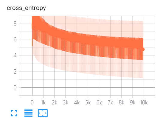
loss = -tf.reduce_sum(Y * tf.log(y_))
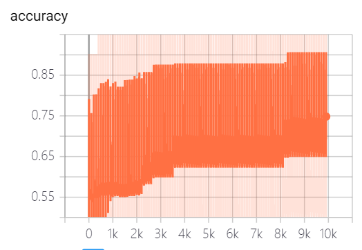
tf.summary.scalar('cross_entropy', loss)
optimizer = tf.train.GradientDescentOptimizer(learning_rate = learning_rate).minimize(loss)
correct_prediction = tf.equal(tf.argmax(y_,1), tf.argmax(Y,1))
accuracy = tf.reduce_mean(tf.cast(correct_prediction, tf.float32))
tf.summary.scalar('accuracy', accuracy)
merged = tf.summary.merge_all()
with tf.Session() as session:
init = tf.global_variables_initializer()
session.run(init)
summary_writer = tf.summary.FileWriter(tensorbardLogPath, session.graph)
for epoch in range(training_epochs):
cost_history = np.empty(shape=[1],dtype=float)
for b in range(total_batchs):
offset = (b * batch_size) % (train_y.shape[0] - batch_size)
batch_x = train_x[offset:(offset + batch_size), :, :, :]
batch_y = train_y[offset:(offset + batch_size), :]
_, c, summary = session.run([optimizer, loss, merged],feed_dict={
X: batch_x, Y : batch_y})
cost_history = np.append(cost_history,c)
summary_writer.add_summary(summary, epoch * training_epochs + b)
print( "Epoch: ",epoch," Training Loss: ",c," Training Accuracy: ",session.run(accuracy, feed_dict={
X: train_x, Y: train_y}))
summary_writer.close()
print( "Testing Accuracy:", session.run(accuracy, feed_dict={
X: test_x, Y: test_y}))
#C:\Users\harry\PycharmProjects\helloworld\cnn_stock
#tensorboard --logdir=log
运行结果
Epoch:  84  Training Loss:  5.750042  Training Accuracy:  0.8020833
Epoch:  85  Training Loss:  5.7415576  Training Accuracy:  0.8020833
Epoch:  86  Training Loss:  5.727802  Training Accuracy:  0.8020833
Epoch:  87  Training Loss:  5.711713  Training Accuracy:  0.8020833
Epoch:  88  Training Loss:  5.6964293  Training Accuracy:  0.8020833
Epoch:  89  Training Loss:  5.693129  Training Accuracy:  0.8020833
Epoch:  90  Training Loss:  5.671862  Training Accuracy:  0.8020833
Epoch:  91  Training Loss:  5.6682425  Training Accuracy:  0.8020833
Epoch:  92  Training Loss:  5.655687  Training Accuracy:  0.8020833
Epoch:  93  Training Loss:  5.638188  Training Accuracy:  0.8020833
Epoch:  94  Training Loss:  5.621099  Training Accuracy:  0.8020833
Epoch:  95  Training Loss:  5.6242228  Training Accuracy:  0.8020833
Epoch:  96  Training Loss:  5.601762  Training Accuracy:  0.8020833
Epoch:  97  Training Loss:  5.590084  Training Accuracy:  0.8020833
Epoch:  98  Training Loss:  5.5816193  Training Accuracy:  0.8020833
Epoch:  99  Training Loss:  5.5780444  Training Accuracy:  0.8020833
Testing Accuracy: 0.6888889