1.软件版本
matlab2015b
2.算法仿真概述
这里,我们的主要算法是结合马尔科夫链-蒙特卡罗方法对先验分布进行抽样,从而确定后验分布的离散值,通过离散值对参数的统计值进行推断。其具体过程如下所示:
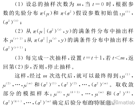
根据所提供的参考文献可知,这里,根据已经得到的先验分布,通过MCMC算法进行抽样,知道完成所有的抽样,通过m次迭代抽样之后,最终确定后验分布。
基本上程序就是按这个步骤进行设计的。
3.部分源码
%Main program
clc;
clear all; % clear the memroy
close all;
warning off;
Num_set = [3];
%为了对比的统一性,将随机化数据进行固定;
rng('default');
nsamples = 2e5;
%%%%%%%%%%%%%%%%%%%%%%%%%%%%%%%%%%%%%%%%%%%%%%%%%%%%%%%%%%%%%%%%%%%%%%%%%%%
%加入参数n的随机化参数,即n为随机的1,2,3,4数据
%initial n,1,2,3,4,........
Num = Num_set(1);
Nn2 = func_differentN(Num,nsamples);
%%%%%%%%%%%%%%%%%%%%%%%%%%%%%%%%%%%%%%%%%%%%%%%%%%%%%%%%%%%%%%%%%%%%%%%%%%%
rng('default');
%%%%%%%%%%%%%%%%%%%%%%%%%%%%%%%%%%%%%%%%%%%%%%%%%%%%%%%%%%%%%%%%%%%%%%%%%%%
%以下几个参数不变,还是使用你的main1种的参数;
D = 458.8; % Diameter of pipe, mm
t = 8.1; % Thickness of defect, mm
D_t = D*t;
sigma_u = 718.2; % Ultimate tensile stress, Mpa
kk = 3; % Number of service years
delT = 1; % Time Interval
do = 5.39; % Intial defect depth mean- mm, N.D
doS = 0.25;% Intial defect depth std -mm,
Lo = 39.6; % Intial defect length - mm, N.D
LoS = 0.25; % Intial defect length std 4
drate = 0.250; % Corrosion depth rate mm/yr - N.D
drateS = 0.04; % Corrosion depth rate Std
Lrate = 20; % Corrosion length rate mm/yr - N.D
LrateS = 10; % Corrosion length rate Std
do1 = normrnd(do,doS,nsamples,1); % Initial defect depth
Lo1 = normrnd(Lo,LoS,nsamples,1); % Initial defect length
%%%%%%%%%%%%%%%%%%%%%%%%%%%%%%%%%%%%%%%%%%%%%%%%%%%%%%%%%%%%%%%%%%%%%%%%%%%
%Calaulate the depth change rate and length change rate with time
for kk1 =1:(kk -1);
drate1 = normrnd(0,drateS, nsamples,1, kk1); % Measured defect depth @ time T
Lrate1 = normrnd(0,LrateS, nsamples,1, kk1); % Measured defect length @ time T
if kk1 == 1
dt(:,:,kk1) = do1(:,:,kk1) + drate1(:,:,kk1)*(delT) ;
dt1(:,:,kk1) = dt(:,:,kk1);
Lt(:,:,kk1) = Lo1(:,:,kk1) + Lrate1(:,:,kk1)*(delT) ;
else
dt(:,:,kk1) = dt(:,:,kk1-1) + drate1(:,:,kk1)*(delT);
dt1(:,:,kk1) = dt(:,:,kk1) ;
Lt(:,:,kk1) = Lt(:,:,kk1-1) + Lrate1(:,:,kk1)*(delT);
end
end
K_d = length(dt(:,:,kk1)); %total number of d
K_l = length(Lt(:,:,kk1)); %total number of l
for i = 1:K_d
if Nn2(i) == 1
dt1(i,:,kk1) = dt1(i,:,kk1);
else
dt1(i,:,kk1) = 5.39 + 0.19*dt1(i,:,kk1) - 0.02*Lt(i,:,kk1) + 0.35*Nn2(i);
end
end
%to obtaion a average number of do_rate and Lo_rate
do_rate = sum(dt1(:,:,kk1))/K_d;
Lo_rate = sum(Lt(:,:,kk1))/K_l;
% Q = sqrt(1+0.31*power(Lo_rate/sqrt(D/t),2));
% Q--length of correction factor
Q1 =(Lo_rate/sqrt(D_t))^2;
Q = sqrt(1+0.31*Q1);
% pf_rate=(2*t*sigma_u*(1-do_rate/t))/(D-t)/(1-(do_rate/t)/Q);
% pf -- failure pressure
pf_rate_1 = 2*t*sigma_u*(1-do_rate/t);
pf_rate_2 =(D-t)*(1-do_rate/t/Q);
pf_rate = pf_rate_1/pf_rate_2;
grid_dist = pf_rate*0.001/20; % in order to get the obvious result on the plot
x = grid_dist:grid_dist:pf_rate*0.015;
%fit the contineous inverted gamma density to the data
par = invgamafit(pf_rate*0.001); % change pf_rate from mPa to kPa, in order to get the obvious result on the plot
a = par(1);
b = 1/par(2);
%Examining inverted gamma distributed prior
prior = exp(a*log(b)-gammaln(a)+(-a-1)*log(x)-b./x);
%Examination of inverted gamma post prior after perfect inspection
A = a + dt1(K_d)/pf_rate^2;
B = b + Lt(K_l)/pf_rate^2;
postprior = exp(A*log(B)-gammaln(A)-(A+1)*log(x)-B./x);
%***********************************************************************************
% % %***********************************************************************************
% %定义likelyhood
% likeliprod = likelihoods(x,t,dt(:,:,kk1),Lt(:,:,kk1),Nn2);
%***********************************************************************************
%这个部分和之前的不一样了,修改后的如下所示:
%***********************************************************************************
%对prior参数进行随机化构造
m = 10;
for ijk = 1:m
ijk
%***********************************************************************************
%***********************************************************************************
%Calaulate the depth change rate and length change rate with time
for kk1 =1:(kk -1);
drate1 = normrnd(0,drateS, nsamples,1, kk1); % Measured defect depth @ time T
Lrate1 = normrnd(0,LrateS, nsamples,1, kk1); % Measured defect length @ time T
if kk1 == 1
dt(:,:,kk1) = do1(:,:,kk1) + drate1(:,:,kk1)*(delT) ;
dt1(:,:,kk1) = dt(:,:,kk1);
Lt(:,:,kk1) = Lo1(:,:,kk1) + Lrate1(:,:,kk1)*(delT) ;
else
dt(:,:,kk1) = dt(:,:,kk1-1) + drate1(:,:,kk1)*(delT);
dt1(:,:,kk1) = dt(:,:,kk1) ;
Lt(:,:,kk1) = Lt(:,:,kk1-1) + Lrate1(:,:,kk1)*(delT);
end
end
K_d = length(dt(:,:,kk1)); %total number of d
K_l = length(Lt(:,:,kk1)); %total number of l
for i = 1:K_d
if Nn2(i) == 1
dt1(i,:,kk1) = dt1(i,:,kk1);
else
dt1(i,:,kk1) = 5.39 + 0.19*dt1(i,:,kk1) - 0.02*Lt(i,:,kk1) + 0.35*Nn2(i);
end
end
%to obtaion a average number of do_rate and Lo_rate
do_rate = sum(dt1(:,:,kk1))/K_d;
Lo_rate = sum(Lt(:,:,kk1))/K_l;
% Q = sqrt(1+0.31*power(Lo_rate/sqrt(D/t),2));
% Q--length of correction factor
Q1 =(Lo_rate/sqrt(D_t))^2;
Q = sqrt(1+0.31*Q1);
% pf_rate=(2*t*sigma_u*(1-do_rate/t))/(D-t)/(1-(do_rate/t)/Q);
% pf -- failure pressure
pf_rate_1 = 2*t*sigma_u*(1-do_rate/t);
pf_rate_2 =(D-t)*(1-do_rate/t/Q);
pf_rate = pf_rate_1/pf_rate_2;
grid_dist = pf_rate*0.001/20; % in order to get the obvious result on the plot
x = grid_dist:grid_dist:pf_rate*0.015;
%fit the contineous inverted gamma density to the data
par = invgamafit(pf_rate*0.001); % change pf_rate from mPa to kPa, in order to get the obvious result on the plot
as(1,ijk) = par(1);
bs(1,ijk) = 1/par(2);
%***********************************************************************************
%***********************************************************************************
end
npar = m; % dimension of the target
drscale = m; % DR shrink factor
adascale = 2.4/sqrt(npar); % scale for adaptation
nsimu = 5e5; % number of simulations
c = 10; % cond number of the target covariance
a = ones(npar,1); % 1. direction
[Sig,Lam]= covcond(c,a); % covariance and its inverse
mu = as;% center point
model.ssfun = inline('(x-d.mu)*d.Lam*(x-d.mu)''','x','d');
params.par0 = mu+0.1; % initial value
params.bounds = (ones(npar,2)*diag([0,Inf]))';
data = struct('mu',mu,'Lam',Lam);
options.nsimu = nsimu;
options.adaptint = 100;
options.qcov = Sig.*2.4^2./npar;
options.drscale = drscale;
options.adascale = adascale; % default is 2.4/sqrt(npar) ;
options.printint = 100;
[Aresults,Achain]= dramrun(model,data,params,options);
mu = bs;% center point
model.ssfun = inline('(x-d.mu)*d.Lam*(x-d.mu)''','x','d');
params.par0 = mu+0.1; % initial value
params.bounds = (ones(npar,2)*diag([0,Inf]))';
data = struct('mu',mu,'Lam',Lam);
options.nsimu = nsimu;
options.adaptint = 100;
options.qcov = Sig.*2.4^2./npar;
options.drscale = drscale;
options.adascale = adascale; % default is 2.4/sqrt(npar) ;
options.printint = 100;
[Bresults,Bchain]= dramrun(model,data,params,options);
%选择值最集中的最为最终的值;
for i = 1:m
[Na,Xa] = hist(Achain(:,i));
[V,I] = max(Na);
A1(i) = Xa(I);
[Nb,Xb] = hist(Bchain(:,i));
[V,I] = max(Nb);
B1(i) = Xb(I);
end
As = mean(A1);
Bs = mean(B1);
post_imp_prior = exp(As*log(Bs)-gammaln(As)-(As+1)*log(x)-Bs./x);
post_imp_prior_CDF = cumsum(post_imp_prior)*grid_dist;
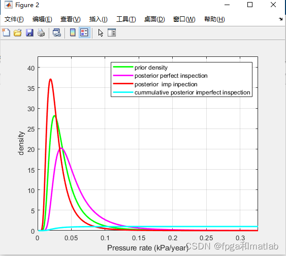
figure
plot(x,prior, 'g-','linewidth',2);
hold on
plot(x, postprior, 'm-','linewidth',2);
hold on
plot(x, post_imp_prior, 'r-','linewidth',2);
hold on
plot(x, post_imp_prior_CDF, 'c-','linewidth',2);
hold on
grid
legend('prior density', 'posterior perfect inspection','posterior imp inpection','cummulative posterior imperfect inspection', 0);
xlabel('Pressure rate (kPa/year)');
ylabel('density');
axis([0,pf_rate*0.015,0,1.15*max([max(prior),max(postprior),max(post_imp_prior),max(post_imp_prior_CDF)])]);
4.仿真结论
5.参考文献
[1]朱新玲. 马尔科夫链蒙特卡罗方法研究综述[J]. 统计与决策, 2009(21):3.A16-51