SSD PyTorch源码解析

0. 引言

0.1 代码来源

代码来源：https://github.com/NVIDIA/DeepLearningExamples/tree/master/PyTorch/Detection/SSD

0.2 代码改动

NVIDIA复现的代码中有很多前沿的新技术（tricks），比如NVIDIA DALI模块，该模块可以加速数据的读取和预处理。注意，虽然NVIDIA复现了该代码，但相关人员对代码进行了修改。

The SSD300 v1.1 model is based on the SSD: Single Shot MultiBox Detector paper, which describes SSD as “a method for detecting objects in images using a single deep neural network". The input size is fixed to 300x300.

输入依然是300×300

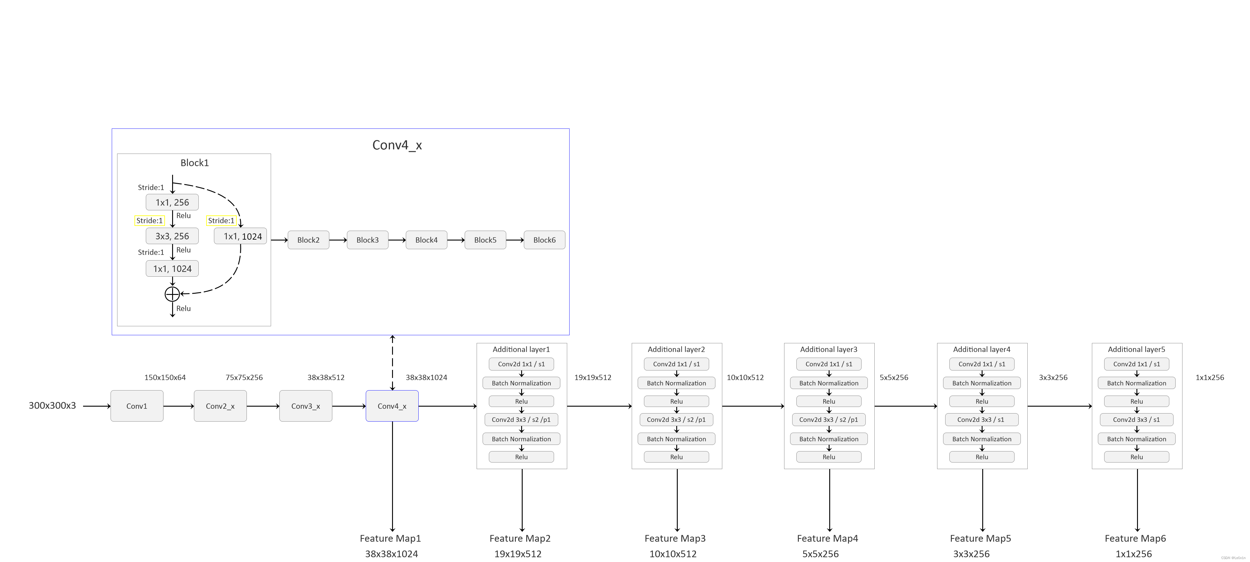
The main difference between this model and the one described in the paper is in the backbone. Specifically, the VGG model is obsolete and is replaced by the ResNet-50 model.

没有继续使用论文中VGG-16作为backbone，而是使用ResNet-50。

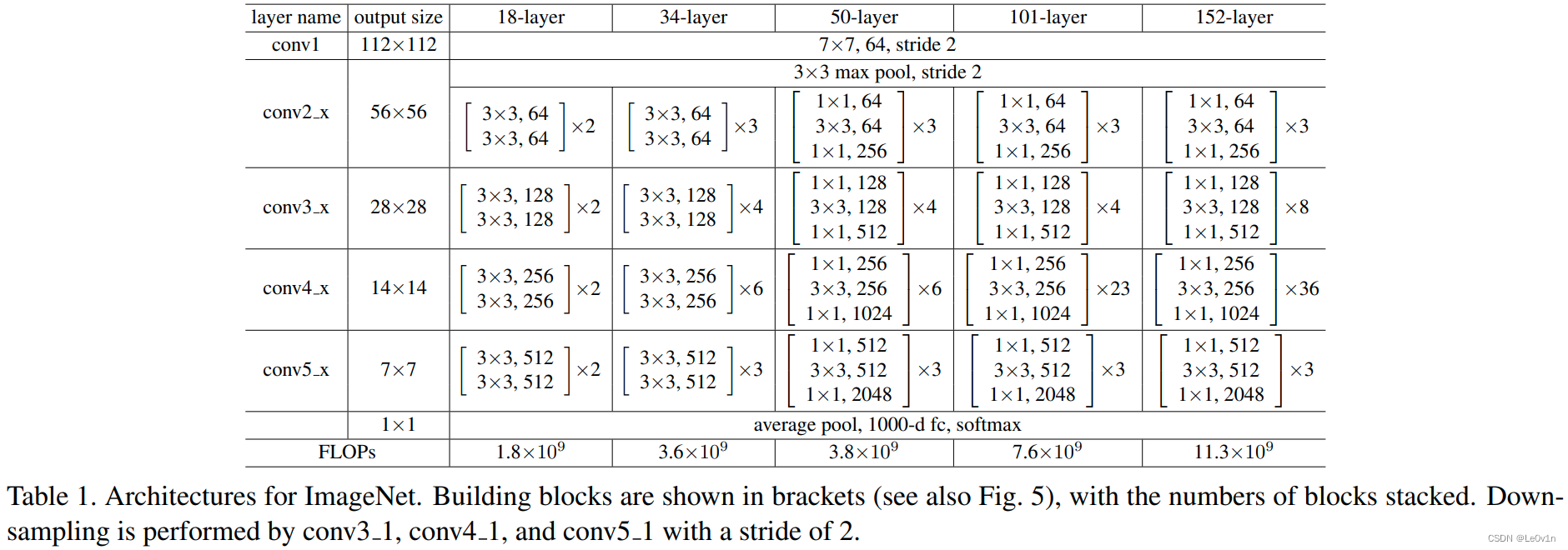
From the Speed/accuracy trade-offs for modern convolutional object detectors paper, the following enhancements were made to the backbone:

• The conv5_x, avgpool, fc and softmax layers were removed from the original classification model.
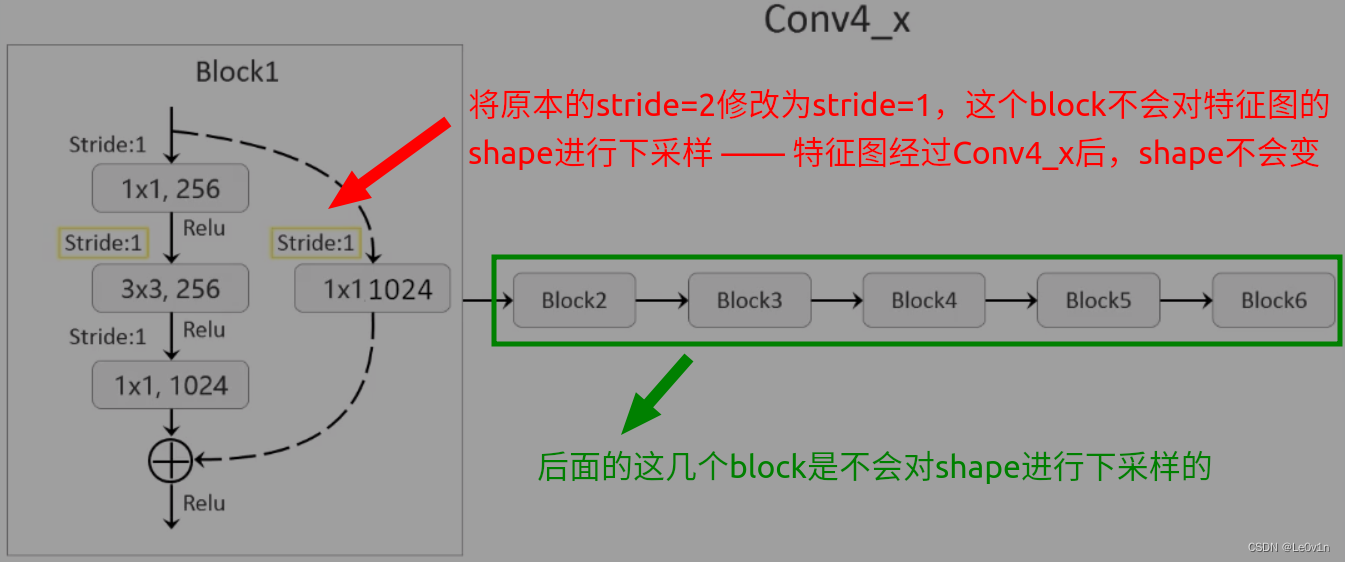
• All strides in conv4_x are set to 1x1.

• 移除ResNet-50最后一个残差结构(conv5_x)以及后面的结构
• 对于conv4_x的第一个残差结构，将其stride都修改为1×1大小 —— 这个残差结构里面有6个block，只有第一个block会对shape进行下采样，而我们只需要修改第一个残差结构的卷积核大小和步距为1 —— 那么特征图在经过这个残差结构后，特征图的shape不会发生变化（不影响通道数，因为通道数=卷积核的个数）
  
  之前在SSD理论上说过，经过backbone之后会让特征图经过一系列的卷积从而生成不同感受野的预测特征图。
  输入图像经过backbone之后会生成第一个预测特征图

Detector heads are similar to the ones referenced in the paper, however, they are enhanced by additional BatchNorm layers after each convolution.

检测器和原论文基本上一样，不同的是在每一个卷积层都引入了额外的BN层（在原论文的中，生成预测特征图的卷积是没有使用BN的）

Additionally, we removed weight decay on every bias parameter and all the BatchNorm layer parameters as described in the Highly Scalable Deep Learning Training System with Mixed-Precision: Training ImageNet in Four Minutes paper.

此外，我们删除了每个偏差参数和所有 BatchNorm 层参数的权重衰减，如具有混合精度的高度可扩展深度学习训练系统：四分钟内训练 ImageNet 论文中所述。

Training of SSD requires computational costly augmentations. To fully utilize GPUs during training we are using the NVIDIA DALI library to accelerate data preparation pipelines.

SSD 的训练需要计算成本高昂的增强。 为了在训练期间充分利用 GPU，我们正在使用 NVIDIA DALI 库来加速数据预处理流程。
我们训练网络的时候基本上使用CPU对数据进行读取和预处理，然后再将数据传入GPUs进行模型的训练。
但这种方法有一个问题：训练模型的时候GPUs的利用率很低。出现这种问题的主要原因是数据的读取和预处理太慢了。CPU处理数据太慢了，而GPUs处理数据又太快了——GPUs处理好了这个batch的数据，而CPU还没准备好下一个batch的数据 —— GPUs空闲 -> 导致GPUs利用率低
针对这个问题，NVIDIA提供了NVIDIA DALI包 —— 让GPUs处理数据

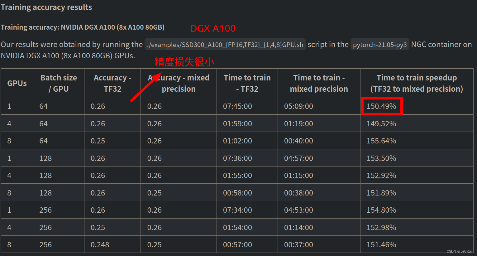
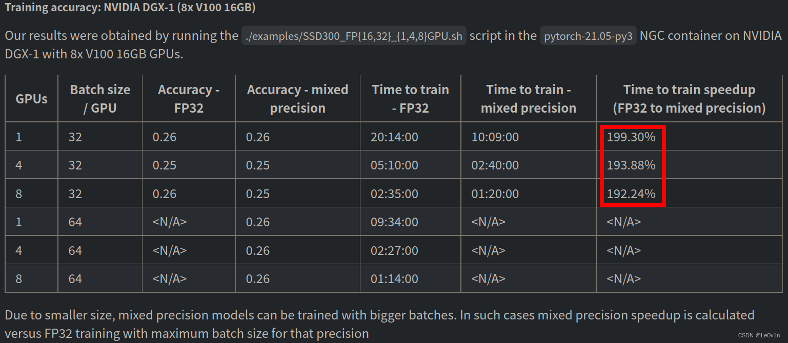
This model is trained with mixed precision using Tensor Cores on Volta, Turing, and the NVIDIA Ampere GPU architectures. Therefore, researchers can get results 2x faster than training without Tensor Cores, while experiencing the benefits of mixed precision training. This model is tested against each NGC monthly container release to ensure consistent accuracy and performance over time.

该模型使用 Volta、Turing 和 NVIDIA Ampere GPU 架构上的 Tensor Cores 以混合精度进行训练。 因此，研究人员可以获得比没有 Tensor Cores 的训练快 2 倍的结果，同时体验混合精度训练的好处。 该模型针对每个 NGC 每月容器版本进行测试，以确保随着时间的推移保持一致的准确性和性能。

0.3 代码使用注意事项

0.3.1 环境配置：

• Python 3.6/3.7/3.8
• Pytorch 1.7.1
• pycocotools(Linux:pip install pycocotools; Windows:pip install pycocotools-windows(不需要额外安装vs))
• Ubuntu或Centos(不建议Windows)
• 最好使用GPU训练

0.3.2 文件结构：

├── src: 实现SSD模型的相关模块    
│     ├── resnet50_backbone.py   使用resnet50网络作为SSD的backbone  
│     ├── ssd_model.py           SSD网络结构文件 
│     └── utils.py               训练过程中使用到的一些功能实现
├── train_utils: 训练验证相关模块（包括cocotools）  
├── my_dataset.py: 自定义dataset用于读取VOC数据集    
├── train_ssd300.py: 以resnet50做为backbone的SSD网络进行训练    
├── train_multi_GPU.py: 针对使用多GPU的用户使用    
├── predict_test.py: 简易的预测脚本，使用训练好的权重进行预测测试    
├── pascal_voc_classes.json: pascal_voc标签文件    
├── plot_curve.py: 用于绘制训练过程的损失以及验证集的mAP
└── validation.py: 利用训练好的权重验证/测试数据的COCO指标，并生成record_mAP.txt文件

0.3.3 预训练权重下载地址（下载后放入src文件夹中）：

• ResNet50+SSD: https://ngc.nvidia.com/catalog/models
  搜索ssd -> 找到SSD for PyTorch(FP32) -> download FP32 -> 解压文件
• 如果找不到可通过百度网盘下载，链接:https://pan.baidu.com/s/1byOnoNuqmBLZMDA0-lbCMQ 提取码:iggj

0.3.4 数据集，本例程使用的是PASCAL VOC2012数据集(下载后放入项目当前文件夹中)

• Pascal VOC2012 train/val数据集下载地址：http://host.robots.ox.ac.uk/pascal/VOC/voc2012/VOCtrainval_11-May-2012.tar
• Pascal VOC2007 test数据集请参考：http://host.robots.ox.ac.uk/pascal/VOC/voc2007/VOCtest_06-Nov-2007.tar

Q：为什么不用MS COCO数据集
A：因为COCO数据集太大了，有几十个G -> 训练时间太长太昂贵

0.3.5 训练方法

• 确保提前准备好数据集
• 确保提前下载好对应预训练模型权重
• 单GPU训练或CPU，直接使用train_ssd300.py训练脚本
• 若要使用多GPU训练，使用 python -m torch.distributed.launch --nproc_per_node=8 --use_env train_multi_GPU.py 指令

nproc_per_node参数为使用GPU数量

0.3.6 训练结果展示

因为多次训练花费的时间太多（训练集为VOC 2012），所以这里只训练了5个epoch，结果如下：

Accumulating evaluation results...
DONE (t=2.50s).
IoU metric: bbox
 Average Precision  (AP) @[ IoU=0.50:0.95 | area=   all | maxDets=100 ] = 0.295
 Average Precision  (AP) @[ IoU=0.50      | area=   all | maxDets=100 ] = 0.567
 Average Precision  (AP) @[ IoU=0.75      | area=   all | maxDets=100 ] = 0.273
 Average Precision  (AP) @[ IoU=0.50:0.95 | area= small | maxDets=100 ] = 0.051
 Average Precision  (AP) @[ IoU=0.50:0.95 | area=medium | maxDets=100 ] = 0.158
 Average Precision  (AP) @[ IoU=0.50:0.95 | area= large | maxDets=100 ] = 0.355
 Average Recall     (AR) @[ IoU=0.50:0.95 | area=   all | maxDets=  1 ] = 0.323
 Average Recall     (AR) @[ IoU=0.50:0.95 | area=   all | maxDets= 10 ] = 0.449
 Average Recall     (AR) @[ IoU=0.50:0.95 | area=   all | maxDets=100 ] = 0.459
 Average Recall     (AR) @[ IoU=0.50:0.95 | area= small | maxDets=100 ] = 0.112
 Average Recall     (AR) @[ IoU=0.50:0.95 | area=medium | maxDets=100 ] = 0.311
 Average Recall     (AR) @[ IoU=0.50:0.95 | area= large | maxDets=100 ] = 0.520
successful save loss curve! 
successful save mAP curve!

SSD算法和Faster R-CNN检测精度差不多。对于小的数据集，Faster R-CNN的检测精度应该比SSD高；当数据集很大时，Faster R-CNN和SSD的检测精度是差不多的。
SSD的检测速度比Faster R-CNN要快很多

• Faster R-CNN在单张GPU上大概每秒能检测6~7张图片
• SSD在单张GPU上大概每秒能检测50~60张图片

Note：

• 相比使用了FPN（特征金字塔）的Faster R-CNN而言，SSD的检测精度要差很多
• 但后面有一个模型是SSD+FPN，名为RetinaNet -> 使用ResNet和FPN作为检测模型的backbone，相比使用了FPN的Faster R-CNN而言，检测精度差不多，但速度提升很多
• 对于我们真正的生产环境，如果真的要使用目标检测模型其实还需要做很多后续的工作。
  + 模式使用GPU进行训练，需将模型转换为TensorRT的格式（检测速度还会提升）

1. SSD代码

1.1 框架示意图

1.2 SSD网络的搭建 —— ssd_model.py

1.2.1 修改backbone（ResNet-50）

class Backbone(nn.Module):
    def __init__(self, pretrain_path=None):
        super(Backbone, self).__init__()
        net = resnet50()
        self.out_channels = [1024, 512, 512, 256, 256, 256]  # 对应每一个预测特征图的channels

        if pretrain_path is not None:
            net.load_state_dict(torch.load(pretrain_path))

        # 构建backbone（截止到conv4_x）
        """
            net.children():
                net: 实例化的ResNet-50网络
                children()：网络下一层所有的子模块（简单理解为，只要是`nn.xxx`构建的层结构都可以认为是它的子模块）
            
            *list(net.children())[:7]
                先将net.children()得到的子模块使用list接收
                对list进行切片，只取前7个子模块（0, 1, 2, ..., 6）
                    ① conv1; ② bn1; ③ relu; ④ maxpool; ⑤ layer1; ⑥ layer2; ⑦ layer3
                再将list进行解包送给nn.Sequential完成网络的重构（后面的就都不要了）
        """
        self.feature_extractor = nn.Sequential(*list(net.children())[:7])

        # 修改Conv4_x中的第一个block
        conv4_block1 = self.feature_extractor[-1][0]  # -1为最后一个子模块， 0为第一个block

        # 修改conv4_block1的步距，从2->1
        conv4_block1.conv1.stride = (1, 1)  # 1×1卷积的步距  对于ResNet-50没必要，但对于ResNet-18/34是有必要的
        conv4_block1.conv2.stride = (1, 1)  # 3×3卷积的步距
        conv4_block1.downsample[0].stride = (1, 1)  # 捷径路径上的步距

    def forward(self, x):
        x = self.feature_extractor(x)
        return x

1.2.2 搭建SSD网络

class SSD300(nn.Module):
    def __init__(self, backbone=None, num_classes=21):
        super(SSD300, self).__init__()
        if backbone is None:
            raise Exception("backbone is None")
        if not hasattr(backbone, "out_channels"):
            raise Exception("the backbone not has attribute: out_channel")
        self.feature_extractor = backbone
        self.num_classes = num_classes

        # 构建后面一系列的特征提取层（为了生成不同的预测特征图）
        # out_channels = [1024, 512, 512, 256, 256, 256] for resnet50
        self._build_additional_features(self.feature_extractor.out_channels)

        """
            定义预测器：① box回归的预测参数； ② 预测的confidence分数
        """
        self.num_defaults = [4, 6, 6, 6, 4, 4]  # 每一个Default box的scale（即box的生成数量） —— 在每个预测特征图上生成多少个Default Box
        location_extractors = []  # 存储回归预测器
        confidence_extractors = []  # 存储置信度预测器

        # out_channels = [1024, 512, 512, 256, 256, 256] for resnet50
        for nd, oc in zip(self.num_defaults, self.feature_extractor.out_channels):
            # nd is number_default_boxes, oc is output_channel
            location_extractors.append(nn.Conv2d(oc, nd * 4, kernel_size=3, padding=1))  # ① box回归的预测参数
            confidence_extractors.append(nn.Conv2d(oc, nd * self.num_classes, kernel_size=3, padding=1))  # ② 预测的confidence分数

        self.loc = nn.ModuleList(location_extractors)
        self.conf = nn.ModuleList(confidence_extractors)

        # 权重初始化
        self._init_weights()

        default_box = dboxes300_coco()
        self.compute_loss = Loss(default_box)
        self.encoder = Encoder(default_box)
        self.postprocess = PostProcess(default_box)

    def _build_additional_features(self, input_size):
        """
        为backbone(resnet50)添加额外的一系列卷积层，得到相应的一系列特征提取器
        :param input_size:
        :return:
        """
        additional_blocks = []
        # input_size = [1024, 512, 512, 256, 256, 256] for resnet50
        middle_channels = [256, 256, 128, 128, 128]  # 对应5个额外添加层结构的输入通道数
        """
            input_size[:-1]: [1024, 512, 512, 256, 256]  左闭右开，最后一个索引不会取到
            input_size[1:]：[512, 512, 256, 256, 256]  第一个不会取到
        """
        for i, (input_ch, output_ch, middle_ch) in enumerate(zip(input_size[:-1], input_size[1:], middle_channels)):
            padding, stride = (1, 2) if i < 3 else (0, 1)  # 前三个索引,padding=1, stride=2; 最后两个索引：padding=0, stride=1
            layer = nn.Sequential(
                nn.Conv2d(input_ch, middle_ch, kernel_size=1, bias=False),  # 因为使用了BN层，所以将bias设置为False
                nn.BatchNorm2d(middle_ch),
                nn.ReLU(inplace=True),
                # 迭代结果不同就是这个卷积的stride和padding
                nn.Conv2d(middle_ch, output_ch, kernel_size=3, padding=padding, stride=stride, bias=False),  # 因为使用了BN层，所以将bias设置为False
                nn.BatchNorm2d(output_ch),
                nn.ReLU(inplace=True),
            )
            additional_blocks.append(layer)
        self.additional_blocks = nn.ModuleList(additional_blocks)

    def _init_weights(self):
        layers = [*self.additional_blocks, *self.loc, *self.conf]
        for layer in layers:
            for param in layer.parameters():
                if param.dim() > 1:
                    nn.init.xavier_uniform_(param)

    # Shape the classifier to the view of bboxes
    def bbox_view(self, features, loc_extractor, conf_extractor):
        """
            通过bbox_view()这个方法得到所有预测特征图上预测的回归参数和置信度得分
                参数：
                    detection_features：预测特征图的list
                    self.loc: 回归预测器
                    self.conf: 置信度预测器
                返回值：
                    locs： 每个box的回归参数
                    confs：每个box的类别（置信度）分数
        """
        locs = []
        confs = []
        for f, l, c in zip(features, loc_extractor, conf_extractor):
            # [batch, n*4, feat_size, feat_size] -> [batch, 4, -1] = [BS, 4, n*feat_size*feat_size]
            # [BS, 4, n*feat_size*feat_size] = [BS, 4个回归参数, 当前预测特征图所有的Default box数量]
            # l(f) -> 得到location回归参数
            locs.append(l(f).view(f.size(0), 4, -1))

            # [batch, n*classes, feat_size, feat_size] -> [batch, classes, -1] -> [BS, classes, n*feat_size*feat_size]
            # c(f) -> 得到confidence参数
            confs.append(c(f).view(f.size(0), self.num_classes, -1))

        """
            使用view()方法时并不会改变原始数据存储的方式，所以需要调用contiguous()来将数据调整为存储连续的tensor
        """
        locs, confs = torch.cat(locs, 2).contiguous(), torch.cat(confs, 2).contiguous()
        return locs, confs

    def forward(self, image, targets=None):
        # image：打包好的一批图片数据
        x = self.feature_extractor(image)  # [1024, 38, 38]

        # Feature Map 38x38x1024, 19x19x512, 10x10x512, 5x5x256, 3x3x256, 1x1x256
        detection_features = torch.jit.annotate(List[Tensor], [])  # [x]  # 存储每一个预测特征图的list
        detection_features.append(x)  # Feature Map1添加到list中
        # 遍历得到Feature Map2~6
        for layer in self.additional_blocks:
            x = layer(x)
            detection_features.append(x)

        """
            通过bbox_view()这个方法得到所有预测特征图上预测的回归参数和置信度得分
                参数：
                    detection_features：预测特征图的list
                    self.loc: 回归预测器
                    self.conf: 置信度预测器
                返回值：
                    locs： 每个box的回归参数
                    confs：每个box的类别（置信度）分数
        """
        # Feature Map 38x38x4, 19x19x6, 10x10x6, 5x5x6, 3x3x4, 1x1x4
        locs, confs = self.bbox_view(detection_features, self.loc, self.conf)

        # For SSD 300, shall return nbatch x 8732 x {nlabels, nlocs} results
        # 38x38x4 + 19x19x6 + 10x10x6 + 5x5x6 + 3x3x4 + 1x1x4 = 8732

        """
            如果是训练模式，则会进一步计算损失（不进行后处理）
            如果是eval模式，直接进行后处理（不进行损失计算），得到最终的结果
        """
        if self.training:
            if targets is None:
                raise ValueError("In training mode, targets should be passed")
            # bboxes_out (Tensor 8732 x 4), labels_out (Tensor 8732)
            bboxes_out = targets['boxes']
            bboxes_out = bboxes_out.transpose(1, 2).contiguous()
            # print(bboxes_out.is_contiguous())
            labels_out = targets['labels']
            # print(labels_out.is_contiguous())

            # ploc, plabel, gloc, glabel
            loss = self.compute_loss(locs, confs, bboxes_out, labels_out)
            return {
    
    "total_losses": loss}

        # 将预测回归参数叠加到default box上得到最终预测box，并执行非极大值抑制虑除重叠框
        # results = self.encoder.decode_batch(locs, confs)
        results = self.postprocess(locs, confs)
        return results

1.3 Default Box的生成

def dboxes300_coco():
    figsize = 300  # 输入网络的图像大小
    feat_size = [38, 19, 10, 5, 3, 1]   # 每个预测层的feature map尺寸
    steps = [8, 16, 32, 64, 100, 300]   # 每个特征层上的一个cell在原图上的跨度
    # use the scales here: https://github.com/amdegroot/ssd.pytorch/blob/master/data/config.py
    scales = [21, 45, 99, 153, 207, 261, 315]  # 每个特征层上预测的default box的scale
    aspect_ratios = [[2], [2, 3], [2, 3], [2, 3], [2], [2]]  # 每个预测特征层上预测的default box的ratios
    dboxes = DefaultBoxes(figsize, feat_size, steps, scales, aspect_ratios)
    return dboxes

class DefaultBoxes(object):
    """
        这个类专门用来生成Default Box
            参数：
                fig_size：输入网络的图片大小 -> 300
                feat_size：每个预测特征图的尺寸(6个预测特征图 -> [38, 19, 10, 5, 3, 1])
                step: 每个在预测特征图上的cell在原图上的跨度 -> [8, 16, 32, 64, 100, 300]
                scales: 就是理论部分讲的scale -> [21, 45, 99, 153, 207, 261, 315]
                aspect_ratio: 每个预测特征图所使用的比例 -> [[2], [2, 3], [2, 3], [2, 3], [2], [2]]
                    有6个预测特征图，所以这个大的list有6个元素
                    为了方便就没有把1:1这个比例写进去
                scale_xy, scale_wh: 在论文中没有提到，但在源码是有这两个参数的。 可以理解为是一个trick，在损失函数部分会进一步讲解
    """
    def __init__(self, fig_size, feat_size, steps, scales, aspect_ratios, scale_xy=0.1, scale_wh=0.2):
        self.fig_size = fig_size   # 输入网络的图像大小 300
        # [38, 19, 10, 5, 3, 1]
        self.feat_size = feat_size  # 每个预测层的feature map尺寸

        self.scale_xy_ = scale_xy
        self.scale_wh_ = scale_wh

        # According to https://github.com/weiliu89/caffe
        # Calculation method slightly different from paper
        # [8, 16, 32, 64, 100, 300]
        self.steps = steps    # 每个特征层上的一个cell在原图上的跨度

        # [21, 45, 99, 153, 207, 261, 315]
        self.scales = scales  # 每个特征层上预测的default box的scale

        fk = fig_size / np.array(steps)     # 计算每层特征层的fk
        # [[2], [2, 3], [2, 3], [2, 3], [2], [2]]
        self.aspect_ratios = aspect_ratios  # 每个预测特征层上预测的default box的ratios

        self.default_boxes = []  # 存储后面生成的Default box的坐标信息
        # size of feature and number of feature
        # 遍历每层特征层，计算default box
        for idx, sfeat in enumerate(self.feat_size):
            sk1 = scales[idx] / fig_size  # scale转为相对值[0-1]
            sk2 = scales[idx + 1] / fig_size  # scale转为相对值[0-1]
            sk3 = sqrt(sk1 * sk2)
            # 先添加两个1:1比例的default box宽和高
            """
                添加了2个尺度的Default box
                    尺度为sk1，比例为sk1:sk1 -> 1:1的Default box
                    尺度为sk3，比例为sk3:sk3 -> 1:1的Default box
            """
            all_sizes = [(sk1, sk1), (sk3, sk3)]

            # 再将剩下不同比例的default box宽和高添加到all_sizes中
            for alpha in aspect_ratios[idx]:
                w, h = sk1 * sqrt(alpha), sk1 / sqrt(alpha)  # sk1 * 根号2 / sk1 /根号2 = 2
                all_sizes.append((w, h))  # 2: 1
                all_sizes.append((h, w))  # 1: 2

            # 计算当前特征层对应原图上的所有default box
            for w, h in all_sizes:
                """
                    >>> import itertools
                    >>> for i, j in itertools.product(range(3), repeat=2):\
                    ... print((i, j))
                    ... 
                    (0, 0)  # 第0行的第0个cell
                    (0, 1)  # 第0行的第1个cell
                    (0, 2)  # 第0行的第2个cell
                    (1, 0)  # 第1行的第0个cell
                    (1, 1)  # 第1行的第1个cell
                    (1, 2)
                    (2, 0)
                    (2, 1)
                    (2, 2)
                """
                # 遍历每一个预测特征图的坐标
                for i, j in itertools.product(range(sfeat), repeat=2):  # i -> 行（y）， j -> 列（x）
                    # 计算每个default box的中心坐标（范围是在0-1之间）
                    """
                        Q：为什么i和j要加0.5
                        A：这是因为i和j说白了就是预测特征图上每一个像素点的坐标，像素点长为1宽也为1（这就是一个cell），这个没有什么问题
                           我们想要知道这个cell的中心坐标，而在图像中，坐标原点是在左上角，横坐标向右为正，纵坐标向下为正
                           所以i+0.5就是这个cell的行坐标，j+0.5就是这个cell的纵坐标
                        
                    """
                    # fk是每个预测特征图的feature size
                    cx, cy = (j + 0.5) / fk[idx], (i + 0.5) / fk[idx]
                    self.default_boxes.append((cx, cy, w, h))  # 中心点坐标、宽高都是相对坐标
            """
                为什么要转换为相对值？
                    因为转换为相对值之后，这个坐标就可以应用到不同的预测特征图，或者原图上都行
            """

        # 将default_boxes转为tensor格式
        self.dboxes = torch.as_tensor(self.default_boxes, dtype=torch.float32)  # 这里不转类型会报错
        self.dboxes.clamp_(min=0, max=1)  # 将坐标（x, y, w, h）都限制在0-1之间

        # For IoU calculation
        # ltrb is left top coordinate and right bottom coordinate
        # 将(x, y, w, h)转换成(xmin, ymin, xmax, ymax)，方便后续计算IoU(匹配正负样本时)
        self.dboxes_ltrb = self.dboxes.clone()  # torch.Size([8732, 4]) -> 生成8732个Default box，每个Default box有4个坐标(x,y,w,h)
        self.dboxes_ltrb[:, 0] = self.dboxes[:, 0] - 0.5 * self.dboxes[:, 2]   # xmin <- x - w/2 = 左上角的x坐标
        self.dboxes_ltrb[:, 1] = self.dboxes[:, 1] - 0.5 * self.dboxes[:, 3]   # ymin <- y - h/2 = 左上角的y坐标
        self.dboxes_ltrb[:, 2] = self.dboxes[:, 0] + 0.5 * self.dboxes[:, 2]   # xmax <- w + w/2 = 右下角的x坐标
        self.dboxes_ltrb[:, 3] = self.dboxes[:, 1] + 0.5 * self.dboxes[:, 3]   # ymax <- h + h/2 = 右下角的y坐标
        """
            self.dboxes: x,y,w,h
            self.dboxes_ltrb: x1,y1,x2,y2
        """

    @property
    def scale_xy(self):
        return self.scale_xy_

    @property
    def scale_wh(self):
        return self.scale_wh_

    def __call__(self, order='ltrb'):
        # 根据需求返回对应格式的default box
        if order == 'ltrb':
            return self.dboxes_ltrb

        if order == 'xywh':
            return self.dboxes

1.4 正负样本匹配

class AssignGTtoDefaultBox(object):
    """将DefaultBox与GT进行匹配"""
    def __init__(self):
        self.default_box = dboxes300_coco()  # 创建DBox(最原生的8732）
        self.encoder = Encoder(self.default_box)

    def __call__(self, image, target):
        boxes = target['boxes']  # GTBox的坐标信息
        labels = target["labels"]  # GTBox对应的labels
        # bboxes_out (Tensor 8732 x 4), labels_out (Tensor 8732)
        # 通过self.encoder.encode()方法将DBox与GTBox进行匹配
        bboxes_out, labels_out = self.encoder.encode(boxes, labels)
        target['boxes'] = bboxes_out
        target['labels'] = labels_out

        return image, target


# This function is from https://github.com/kuangliu/pytorch-ssd.
class Encoder(object):
    """
        Inspired by https://github.com/kuangliu/pytorch-src
        Transform between (bboxes, lables) <-> SSD output

        dboxes: default boxes in size 8732 x 4,
            encoder: input ltrb format, output xywh format
            decoder: input xywh format, output ltrb format

        encode:
            input  : bboxes_in (Tensor nboxes x 4), labels_in (Tensor nboxes)
            output : bboxes_out (Tensor 8732 x 4), labels_out (Tensor 8732)
            criteria : IoU threshold of bboexes

        decode:
            input  : bboxes_in (Tensor 8732 x 4), scores_in (Tensor 8732 x nitems)
            output : bboxes_out (Tensor nboxes x 4), labels_out (Tensor nboxes)
            criteria : IoU threshold of bboexes
            max_output : maximum number of output bboxes
    """
    def __init__(self, dboxes):
        self.dboxes = dboxes(order='ltrb')
        self.dboxes_xywh = dboxes(order='xywh').unsqueeze(dim=0)
        self.nboxes = self.dboxes.size(0)  # default boxes的数量
        self.scale_xy = dboxes.scale_xy
        self.scale_wh = dboxes.scale_wh

    def encode(self, bboxes_in, labels_in, criteria=0.5):
        """
        encode:
            input  : bboxes_in (Tensor nboxes x 4), labels_in (Tensor nboxes)
            output : bboxes_out (Tensor 8732 x 4), labels_out (Tensor 8732)
            criteria : IoU threshold of bboexes

            bboxes_in: GTBox的坐标信息
            labels_in： GTBox的标签信息
        """
        # 计算每个GT与default box的iou数值
        ious = calc_iou_tensor(bboxes_in, self.dboxes)  # [GTBox, 8732]

        # 寻找每个default box匹配到的最大IoU: ① 值； ② 对应的索引
        best_dbox_ious, best_dbox_idx = ious.max(dim=0)  # [8732,]

        # 寻找每个GT匹配到的最大IoU
        best_bbox_ious, best_bbox_idx = ious.max(dim=1)  # [GTBox,]

        # 将每个GT匹配到的最佳default box设置为正样本（对应论文中Matching strategy的第一条）
        """
            Matching strategy：
                1. 用每一个GTBox与DBox求IoU（会将GTBox分配给与它IoU最大的DBox）
                2. 将IoU大于0.5的DBox设置为正样本
        """
        # set best ious 2.0
        # 将每个GTBox匹配到的最大IoU的DBox设置为正样本
        """
            tensor.index_fill_(0, best_bbox_idx, 2.0):
                第一个参数： dim
                第二个参数： 需要填充的索引
                第三个参数： 需要填充的数值
            填充的数只要大于0.5都是可以的
        """
        best_dbox_ious.index_fill_(0, best_bbox_idx, 2.0)  # dim, index, value

        # 将相应default box匹配最大IOU的GT索引进行替换  -> best_bbox_idx.size(0): GTBox的数量
        idx = torch.arange(0, best_bbox_idx.size(0), dtype=torch.int64)  # [0, 1, 2, ..., GTBox的数量-1]
        best_dbox_idx[best_bbox_idx[idx]] = idx
        """
            做完上面这两个操作：
                best_dbox_idx和best_bbox_idx的对应关系就一致了
        """

        # filter IoU > 0.5
        # 寻找与GT iou大于0.5的default box,对应论文中Matching strategy的第二条(这里包括了第一条匹配到的信息)
        masks = best_dbox_ious > criteria  # [Boolean, Boolean, ...]

        """
            针对每一个Default Box而言，都已经被划分为正负样本了。
            接下来我们需要对划分为正样本的DBox所对应的GT的 标签和GTBox信息 提取出来，方法后续计算
            
            self.nboxes: DBox的数量
            labels_in：针对每一个GTBox的类别标签
            
            best_dbox_idx[masks]：将mask所有为True的数据取出来 -> 将划分为正样本的所有DBox对应的GTBox的索引取出来
            labels_in[best_dbox_idx[masks]]：再将对应GTBox的索引传去label_in中 -> 所有DBox对应GTBox的标签取出来
            
            在labels_in中，所有正样本的数值>0，所有负样本的数值=0（背景）
            
            这里找正样本DBox对应GTBox的标签，目的是找到DBox的标签（二者是一样的）
        """
        # [8732,]
        labels_out = torch.zeros(self.nboxes, dtype=torch.int64)  # nboxes = DBox
        labels_out[masks] = labels_in[best_dbox_idx[masks]]

        """
            上面两步将所有划分为正样本的DBox的标签取出来了，接下来我们还需要DBox对应GTBox的信息提出来（坐标信息）
            best_dbox_idx[masks]：拿到所有被划分到正样本的GTBox的索引
            bboxes_in[best_dbox_idx[masks]: 拿到针对每一个划分为正样本的DBox所对应GTBox的坐标信息
            (bboxes_in是GTBox的坐标信息)
            
            对于每一个DBox而言，如果它被划分为正样本，那么它的标签和坐标信息都是对应GTBox的标签和坐标的
                             如果它被划分为负样本的话，它的标签为0，它的坐标信息还是它原来的DBox坐标信息
        """
        # 将default box匹配到正样本的位置设置成对应GT的box信息
        bboxes_out = self.dboxes.clone()
        bboxes_out[masks, :] = bboxes_in[best_dbox_idx[masks], :]

        # Transform format to xywh format
        x = 0.5 * (bboxes_out[:, 0] + bboxes_out[:, 2])  # x
        y = 0.5 * (bboxes_out[:, 1] + bboxes_out[:, 3])  # y
        w = bboxes_out[:, 2] - bboxes_out[:, 0]  # w
        h = bboxes_out[:, 3] - bboxes_out[:, 1]  # h
        bboxes_out[:, 0] = x
        bboxes_out[:, 1] = y
        bboxes_out[:, 2] = w
        bboxes_out[:, 3] = h
        return bboxes_out, labels_out

    def scale_back_batch(self, bboxes_in, scores_in):
        """
            将box格式从xywh转换回ltrb, 将预测目标score通过softmax处理
            Do scale and transform from xywh to ltrb
            suppose input N x 4 x num_bbox | N x label_num x num_bbox

            bboxes_in: 是网络预测的xywh回归参数
            scores_in: 是预测的每个default box的各目标概率
        """
        if bboxes_in.device == torch.device("cpu"):
            self.dboxes = self.dboxes.cpu()
            self.dboxes_xywh = self.dboxes_xywh.cpu()
        else:
            self.dboxes = self.dboxes.cuda()
            self.dboxes_xywh = self.dboxes_xywh.cuda()

        # Returns a view of the original tensor with its dimensions permuted.
        bboxes_in = bboxes_in.permute(0, 2, 1)
        scores_in = scores_in.permute(0, 2, 1)
        # print(bboxes_in.is_contiguous())

        bboxes_in[:, :, :2] = self.scale_xy * bboxes_in[:, :, :2]   # 预测的x, y回归参数
        bboxes_in[:, :, 2:] = self.scale_wh * bboxes_in[:, :, 2:]   # 预测的w, h回归参数

        # 将预测的回归参数叠加到default box上得到最终的预测边界框
        bboxes_in[:, :, :2] = bboxes_in[:, :, :2] * self.dboxes_xywh[:, :, 2:] + self.dboxes_xywh[:, :, :2]
        bboxes_in[:, :, 2:] = bboxes_in[:, :, 2:].exp() * self.dboxes_xywh[:, :, 2:]

        # transform format to ltrb
        l = bboxes_in[:, :, 0] - 0.5 * bboxes_in[:, :, 2]
        t = bboxes_in[:, :, 1] - 0.5 * bboxes_in[:, :, 3]
        r = bboxes_in[:, :, 0] + 0.5 * bboxes_in[:, :, 2]
        b = bboxes_in[:, :, 1] + 0.5 * bboxes_in[:, :, 3]

        bboxes_in[:, :, 0] = l  # xmin
        bboxes_in[:, :, 1] = t  # ymin
        bboxes_in[:, :, 2] = r  # xmax
        bboxes_in[:, :, 3] = b  # ymax

        return bboxes_in, F.softmax(scores_in, dim=-1)

    def decode_batch(self, bboxes_in, scores_in, criteria=0.45, max_output=200):
        # 将box格式从xywh转换回ltrb（方便后面非极大值抑制时求iou）, 将预测目标score通过softmax处理
        bboxes, probs = self.scale_back_batch(bboxes_in, scores_in)

        outputs = []
        # 遍历一个batch中的每张image数据
        for bbox, prob in zip(bboxes.split(1, 0), probs.split(1, 0)):
            bbox = bbox.squeeze(0)
            prob = prob.squeeze(0)
            outputs.append(self.decode_single_new(bbox, prob, criteria, max_output))
        return outputs

    def decode_single_new(self, bboxes_in, scores_in, criteria, num_output=200):
        """
        decode:
            input  : bboxes_in (Tensor 8732 x 4), scores_in (Tensor 8732 x nitems)
            output : bboxes_out (Tensor nboxes x 4), labels_out (Tensor nboxes)
            criteria : IoU threshold of bboexes
            max_output : maximum number of output bboxes
        """
        device = bboxes_in.device
        num_classes = scores_in.shape[-1]

        # 对越界的bbox进行裁剪
        bboxes_in = bboxes_in.clamp(min=0, max=1)

        # [8732, 4] -> [8732, 21, 4]
        bboxes_in = bboxes_in.repeat(1, num_classes).reshape(scores_in.shape[0], -1, 4)

        # create labels for each prediction
        labels = torch.arange(num_classes, device=device)
        labels = labels.view(1, -1).expand_as(scores_in)

        # remove prediction with the background label
        # 移除归为背景类别的概率信息
        bboxes_in = bboxes_in[:, 1:, :]
        scores_in = scores_in[:, 1:]
        labels = labels[:, 1:]

        # batch everything, by making every class prediction be a separate instance
        bboxes_in = bboxes_in.reshape(-1, 4)
        scores_in = scores_in.reshape(-1)
        labels = labels.reshape(-1)

        # remove low scoring boxes
        # 移除低概率目标，self.scores_thresh=0.05
        inds = torch.nonzero(scores_in > 0.05, as_tuple=False).squeeze(1)
        bboxes_in, scores_in, labels = bboxes_in[inds], scores_in[inds], labels[inds]

        # remove empty boxes
        ws, hs = bboxes_in[:, 2] - bboxes_in[:, 0], bboxes_in[:, 3] - bboxes_in[:, 1]
        keep = (ws >= 0.1 / 300) & (hs >= 0.1 / 300)
        keep = keep.nonzero(as_tuple=False).squeeze(1)
        bboxes_in, scores_in, labels = bboxes_in[keep], scores_in[keep], labels[keep]

        # non-maximum suppression
        keep = batched_nms(bboxes_in, scores_in, labels, iou_threshold=criteria)

        # keep only topk scoring predictions
        keep = keep[:num_output]
        bboxes_out = bboxes_in[keep, :]
        scores_out = scores_in[keep]
        labels_out = labels[keep]

        return bboxes_out, labels_out, scores_out

    # perform non-maximum suppression
    def decode_single(self, bboxes_in, scores_in, criteria, max_output, max_num=200):
        """
        decode:
            input  : bboxes_in (Tensor 8732 x 4), scores_in (Tensor 8732 x nitems)
            output : bboxes_out (Tensor nboxes x 4), labels_out (Tensor nboxes)
            criteria : IoU threshold of bboexes
            max_output : maximum number of output bboxes
        """
        # Reference to https://github.com/amdegroot/ssd.pytorch
        bboxes_out = []
        scores_out = []
        labels_out = []

        # 非极大值抑制算法
        # scores_in (Tensor 8732 x nitems), 遍历返回每一列数据，即8732个目标的同一类别的概率
        for i, score in enumerate(scores_in.split(1, 1)):
            # skip background
            if i == 0:
                continue

            # [8732, 1] -> [8732]
            score = score.squeeze(1)

            # 虑除预测概率小于0.05的目标
            mask = score > 0.05
            bboxes, score = bboxes_in[mask, :], score[mask]
            if score.size(0) == 0:
                continue

            # 按照分数从小到大排序
            score_sorted, score_idx_sorted = score.sort(dim=0)

            # select max_output indices
            score_idx_sorted = score_idx_sorted[-max_num:]
            candidates = []

            while score_idx_sorted.numel() > 0:
                idx = score_idx_sorted[-1].item()
                # 获取排名前score_idx_sorted名的bboxes信息 Tensor:[score_idx_sorted, 4]
                bboxes_sorted = bboxes[score_idx_sorted, :]
                # 获取排名第一的bboxes信息 Tensor:[4]
                bboxes_idx = bboxes[idx, :].unsqueeze(dim=0)
                # 计算前score_idx_sorted名的bboxes与第一名的bboxes的iou
                iou_sorted = calc_iou_tensor(bboxes_sorted, bboxes_idx).squeeze()

                # we only need iou < criteria
                # 丢弃与第一名iou > criteria的所有目标(包括自己本身)
                score_idx_sorted = score_idx_sorted[iou_sorted < criteria]
                # 保存第一名的索引信息
                candidates.append(idx)

            # 保存该类别通过非极大值抑制后的目标信息
            bboxes_out.append(bboxes[candidates, :])   # bbox坐标信息
            scores_out.append(score[candidates])       # score信息
            labels_out.extend([i] * len(candidates))   # 标签信息

        if not bboxes_out:  # 如果为空的话，返回空tensor，注意boxes对应的空tensor size，防止验证时出错
            return [torch.empty(size=(0, 4)), torch.empty(size=(0,), dtype=torch.int64), torch.empty(size=(0,))]

        bboxes_out = torch.cat(bboxes_out, dim=0).contiguous()
        scores_out = torch.cat(scores_out, dim=0).contiguous()
        labels_out = torch.as_tensor(labels_out, dtype=torch.long)

        # 对所有目标的概率进行排序（无论是什 么类别）,取前max_num个目标
        _, max_ids = scores_out.sort(dim=0)
        max_ids = max_ids[-max_output:]
        return bboxes_out[max_ids, :], labels_out[max_ids], scores_out[max_ids]

1.5 Loss的计算

class Loss(nn.Module):
    """
        Implements the loss as the sum of the followings:
        1. Confidence Loss: All labels, with hard negative mining
        2. Localization Loss: Only on positive labels
        Suppose input dboxes has the shape 8732x4
    """
    def __init__(self, dboxes):
        """
        Args:
            dboxes:  utils中的 dboxes = DefaultBoxes(figsize, feat_size, steps, scales, aspect_ratios)
                即实例化的Default Box

            dboxes.scale_xy = 0.1
            dboxes.scale_wh = 0.2
        """
        super(Loss, self).__init__()
        # Two factor are from following links
        # http://jany.st/post/2017-11-05-single-shot-detector-ssd-from-scratch-in-tensorflow.html
        self.scale_xy = 1.0 / dboxes.scale_xy  # 10
        self.scale_wh = 1.0 / dboxes.scale_wh  # 5

        # 定义计算定位的损失器 -> SmoothL1
        self.location_loss = nn.SmoothL1Loss(reduction='none')

        """
            nn.Parameter：转化为PyTorch的参数
                参数：
                    ① data (Tensor) – parameter tensor.
                    ② requires_grad (bool, optional)    -> Default: True
                        if the parameter requires gradient. 
                        See Locally disabling gradient computation for more details. 
        """
        # [num_anchors, 4] -> [4, num_anchors] -> [1, 4, num_anchors]
        self.dboxes = nn.Parameter(dboxes(order="xywh").transpose(0, 1).unsqueeze(dim=0), requires_grad=False)

        # 定义计算分类的损失器 -> Softmax + 交叉熵
        self.confidence_loss = nn.CrossEntropyLoss(reduction='none')

    def _location_vec(self, loc):
        # type: (Tensor) -> Tensor
        r"""
        - Generate Location Vectors —— 计算ground truth相对anchors的回归参数

        :param loc: anchor匹配到的对应GTBOX Nx4x8732

        计算公式：
            .. math::
                \begin{aligned}
                    & x_{回归} = \frac{x_{gtbox} - x_{dbox}}{w_{dbox}} \\
                    & y_{回归} = \frac{y_{gtbox} - y_{dbox}}{h_{dbox}} \\
                    & w_{回归} = \ln(\frac{w_{gtbox}}{w_{dbox}}) \\
                    & h_{回归} = \ln(\frac{h_{gtbox}}{h_{dbox}}) \\
                \end{aligned}

        .. note::
            - 这里我觉得是计算 `DBox的默认位置` 和 `所匹配到GTBox位置之间` 的差距，拿这个差距和DBox的预测回归参数进行比较，得到损失
            - 也就是说，这里计算的是DBox和GTBox的实际差距（偏离量），网络预测的回归参数是DBox应该位移的量，那这两个数去进行损失函数的计算是比较合理的
            - self.scale_xy（5）和self.scale_wh（10）是两个缩放因子
            - 这么做的原因可以理解为是一个trick -> 加速模型收敛

        :return: 返回DBox与GT的差距，shape为[BS, 4, 8732]
        """
        gxy = self.scale_xy * (loc[:, :2, :] - self.dboxes[:, :2, :]) / self.dboxes[:, 2:, :]  # Nx2x8732
        gwh = self.scale_wh * (loc[:, 2:, :] / self.dboxes[:, 2:, :]).log()  # Nx2x8732
        return torch.cat((gxy, gwh), dim=1).contiguous()

    def forward(self, ploc, plabel, gloc, glabel):
        # type: (Tensor, Tensor, Tensor, Tensor) -> Tensor
        """
            ploc, plabel: Nx4x8732, Nxlabel_numx8732
                predicted location and labels
                ① ploc：预测的回归参数
                ② plabel：预测的标签值

            gloc, glabel: Nx4x8732, Nx8732
                ground truth location and labels
                ① gloc：预处理过程中每个Default Box（这里应该叫anchor）所匹配到的GT box对应的坐标
                ② glabel：预处理过程中每个Default Box（这里应该叫anchor）所匹配到的GT box对应的标签
        """

        """
            在预处理过程中会对每一个Dbox匹配和它对应的GTBox以及标签
                如果该DBox有匹配到GTBox -> 它的glabel肯定是一个>0的数
                如果该DBox没有匹配到GTBox -> 它的glabel被置为0（0对应的是背景）
                
            mask = torch.gt(glabel, 0)
                通过这个运算之后，就能得到所有匹配到GTBox的DBox
                mask是一个蒙版
        """
        # 获取正样本的mask  Tensor: [N, 8732]  N=BS
        mask = torch.gt(glabel, 0)  # (gt: >)
        # mask1 = torch.nonzero(glabel)
        # 计算一个batch中的每张图片的正样本个数 Tensor: [N]
        pos_num = mask.sum(dim=1)  # shape: [BS]：表明是求batch中每张图片正样本的数量
        """
            [ 2, 10, 52, 27]  这里我们的BS=4，所以只有4张图片
                第一张图片匹配到的正样本个数为2
                第二张图片匹配到的正样本个数为10
                ...
        """

        """
            计算每一个DBox所匹配到GTBox的location回归参数
                gloc：预处理过程中每个Default Box所匹配到的GT box对应的坐标
                    shape为[BS, 4, 8732] = [BS, 4个坐标, 所有的DBox]
        """
        # 计算gt的location回归参数 -> 预测框的值 Tensor: [N, 4, 8732]
        vec_gd = self._location_vec(gloc)  # [BS, 4, 8732]

        # sum on four coordinates, and mask
        # 计算定位损失(只有正样本)
        """
            ploc： 预测的回归参数（DBox应该如何移动以更好的匹配GTBox）    [BS, 4, 8732]
            vec_gd：DBox一开始和匹配的的GTBox之间的偏移量              [BS, 4, 8732]
            
            vec_gd计算的是DBox和GTBox的实际差距（偏离量）
            网络预测的回归参数是DBox应该位移的量
            拿这两个数去进行损失函数的计算是比较合理的
            
            Note：
                定位损失应该只计算正样本的定义损失，负样本不应该参与，而loc_loss = self.location_loss(ploc, vec_gd).sum(dim=1)
                计算了所有样本的损失，我们应该对其进行筛选 -> 使用刚才得到mask进行筛选
                    
                    import torch

                    mask = [True, False, True, True, False, False, False, False, True]
                    mask = torch.tensor(mask)
                    
                    mask.float()  # tensor([1., 0., 1., 1., 0., 0., 0., 0., 1.])
        """
        loc_loss = self.location_loss(ploc, vec_gd).sum(dim=1)  # Tensor: [N, 8732]
        loc_loss = (mask.float() * loc_loss).sum(dim=1)  # Tenosr: [N]  -> 对所有的location损失求和 -> 每张图片的location loss

        """
            计算分类损失
                ① plabel： DBox的分类值      torch.Size([4, 21, 8732]) = [BS, classes+1, DBox数量]
                ② glabel： DBox所匹配到的GT的真实分类值     torch.Size([4, 8732]) = [BS, DBox数量]
                    如果该DBox没有匹配到GTBox，则glabel=0（负样本对应的就是背景）
                返回值：
                    con: 每一个DBox的分类损失       torch.Size([4, 8732]) = [BS, DBox数量]
                    
            Note：
                我们不会用到这8732个分类loss的，因为我们在loss时需要考虑到正负样本平衡的问题
                （SSD论文中，正负样本比例为3:1）
                而这8732个DBox只有很少一部分是正样本，绝大多数都是负样本
                如果直接这样计算的话 -> 正负样本不平衡 -> 给网络训练带来很大的困难
                
                所以我们需要分别获取它们的正负样本的loss
                正样本我们一开始就得到了（用mask），现在需要计算负样本
        """
        # hard negative mining Tenosr: [N, 8732]
        con = self.confidence_loss(plabel, glabel)

        # positive mask will never selected
        # 获取负样本
        con_neg = con.clone()
        con_neg[mask] = 0.0  # 将正样本的分类损失全部置为0 -> 得到负样本的分类损失
        # 按照confidence_loss降序排列 con_idx(Tensor: [N, 8732])
        _, con_idx = con_neg.sort(dim=1, descending=True)  # ① 对负样本的分类损失进行降序排列，不要返回值，只要索引 -> 损失越来越小
        _, con_rank = con_idx.sort(dim=1)  # 这个步骤比较巧妙  # ② 对负样本损失的索引进行升序排列

        # number of negative three times positive
        # 用于损失计算的负样本数是正样本的3倍（在原论文Hard negative mining部分），
        # 但不能超过总样本数8732  # mask.size(1)=8732
        neg_num = torch.clamp(3 * pos_num, max=mask.size(1)).unsqueeze(-1)  # 对负样本个数进行限制
        neg_mask = torch.lt(con_rank, neg_num)  # (lt: <) Tensor [N, 8732]  # ③ 进行取值
        """
            经过这①②③三步之后，neg_mask中为True的个数为neg_num，且正好对应分类损失最大的位置
        """

        """
            在得到正负样本的mask之后就可以计算最后的分类损失
                所有的正样本都会用到
                所有总的样本mask = 正样本的mask + 选取的负样本mask -> mask.float() + neg_mask.float()
        """
        # confidence最终loss使用选取的正样本loss+选取的负样本loss
        con_loss = (con * (mask.float() + neg_mask.float())).sum(dim=1)  # Tensor [N]

        """
            总的损失 = (定位损失 + 分类损失) / N
            
            Note:
                N为正样本的个数（而不是总的样本数）
        """
        total_loss = loc_loss + con_loss

        # avoid no object detected
        # 避免出现图像中没有GTBOX的情况
        # eg. [15, 3, 5, 0] -> [1.0, 1.0, 1.0, 0.0]
        """
            pos_num的确是正样本的个数    data: tensor([18, 61,  7,  6], device='cuda:0')
            但是不一定这个batch中每一张图片都有正样本数，因为最后的总损失需要/正样本个数，
            这里总损失是针对一张图片的，而不是一个batch，对于一张图片来说，它的pos_num有可能为0（正样本数为0）
            比如pos_num=tensor([0, 0,  7,  6], device='cuda:0')
            那么在计算时就会出现除零错误，因此需对其下限进行1e-6的限制
        """
        num_mask = torch.gt(pos_num, 0).float()  # 统计一个batch中的每张图像中是否存在正样本， 如果没有则该张图片为负样本，不计算损失
        pos_num = pos_num.float().clamp(min=1e-6)  # 防止出现分母为零的情况
        ret = (total_loss * num_mask / pos_num).mean(dim=0)  # 只计算存在正样本的图像损失
        # ret： tensor(19.5028, device='cuda:0')
        return ret

1.6 后处理 —— 不训练（不计算损失）而是eval模式直接对输出进行后处理

class PostProcess(nn.Module):
    def __init__(self, dboxes):
        """
        如果不在训练，那么就对结果进行后处理
        Args:
            dboxes: 根据预测特征图生成的Default Box（原生的，8732个）
            dboxes_xywh：先对DBox进行调用（格式为xywh），之后再添加一个维度，并且声明它不需要梯度（因为是正向传播不训练），最后将其转换为PyTorch的参数
            dboxes.scale_xy和dboxes.scale_wh是两个超参数
            self.criteria：IoU阈值的标准
            self.max_output: 输出目标的最大数量
        """
        super(PostProcess, self).__init__()
        # [num_anchors, 4] -> [1, num_anchors, 4]
        self.dboxes_xywh = nn.Parameter(dboxes(order='xywh').unsqueeze(dim=0), requires_grad=False)
        self.scale_xy = dboxes.scale_xy  # 0.1
        self.scale_wh = dboxes.scale_wh  # 0.2

        self.criteria = 0.5
        self.max_output = 100

    def scale_back_batch(self, bboxes_in, scores_in):
        # type: (Tensor, Tensor) -> Tuple[Tensor, Tensor]
        """
            1）通过预测的boxes回归参数得到最终预测坐标
            2）将box格式从xywh转换回ltrb（VOC的形式）
            3）将预测目标score通过softmax处理
            Do scale and transform from xywh to ltrb
            suppose input N x 4 x num_bbox | N x label_num x num_bbox

            bboxes_in: [N, 4, 8732]是网络预测的xywh回归参数
            scores_in: [N, label_num, 8732]是预测的每个default box的各目标概率
        """

        # Returns a view of the original tensor with its dimensions permuted.
        # [batch, 4, 8732] -> [batch, 8732, 4]
        bboxes_in = bboxes_in.permute(0, 2, 1)
        # [batch, label_num, 8732] -> [batch, 8732, label_num]  label_num = 20 +1 = 21
        scores_in = scores_in.permute(0, 2, 1)
        # print(bboxes_in.is_contiguous())

        bboxes_in[:, :, :2] = self.scale_xy * bboxes_in[:, :, :2]   # 预测的x, y回归参数
        bboxes_in[:, :, 2:] = self.scale_wh * bboxes_in[:, :, 2:]   # 预测的w, h回归参数

        """
            回归参数的计算如下：
                回归参数x = (GTBox的x - 预测DBox的x) / 预测DBox的w
                回归参数y = (GTBox的y - 预测DBox的y) / 预测DBox的h
                回归参数w = ln(GTBox的w / 预测DBox的w)
                回归参数h = ln(GTBox的h / 预测DBox的h)
                
            现在我们知道回归参数了，去算GTbox：
                GTBox(最终的预测边界框)的x = (回归参数x)*预测DBox的w + 预测DBox的x
                GTBox(最终的预测边界框)的y = (回归参数y)*预测DBox的w + 预测DBox的h
                GTBox(最终的预测边界框)的w = ln(回归参数w) * 预测DBox的w
                GTBox(最终的预测边界框)的h = ln(回归参数h) * 预测DBox的h
        """
        # 将预测的回归参数叠加到default box上得到最终的预测边界框
        bboxes_in[:, :, :2] = bboxes_in[:, :, :2] * self.dboxes_xywh[:, :, 2:] + self.dboxes_xywh[:, :, :2]  # xy
        bboxes_in[:, :, 2:] = bboxes_in[:, :, 2:].exp() * self.dboxes_xywh[:, :, 2:]  # wh

        # transform format to ltrb
        l = bboxes_in[:, :, 0] - 0.5 * bboxes_in[:, :, 2]
        t = bboxes_in[:, :, 1] - 0.5 * bboxes_in[:, :, 3]
        r = bboxes_in[:, :, 0] + 0.5 * bboxes_in[:, :, 2]
        b = bboxes_in[:, :, 1] + 0.5 * bboxes_in[:, :, 3]

        bboxes_in[:, :, 0] = l  # xmin
        bboxes_in[:, :, 1] = t  # ymin
        bboxes_in[:, :, 2] = r  # xmax
        bboxes_in[:, :, 3] = b  # ymax

        # scores_in: [batch, 8732, label_num]
        return bboxes_in, F.softmax(scores_in, dim=-1)

    def decode_single_new(self, bboxes_in, scores_in, criteria, num_output):
        # type: (Tensor, Tensor, float, int) -> Tuple[Tensor, Tensor, Tensor]
        """
        decode:
            input  : bboxes_in (Tensor 8732 x 4), scores_in (Tensor 8732 x nitems)
            output : bboxes_out (Tensor nboxes x 4), labels_out (Tensor nboxes)
            criteria : IoU threshold of bboexes
            max_output : maximum number of output bboxes
        """
        device = bboxes_in.device  # 获取变量的设备信息
        num_classes = scores_in.shape[-1]  # 类别个数（20 + 1 = 21）

        # 对越界的bbox进行裁剪
        """
            Note: 这里bboxes_in里面的都是相对值，所以将其限制在[0, 1]就可以了
        """
        bboxes_in = bboxes_in.clamp(min=0, max=1)

        """
            SSD算法每一个DBox只预测一组回归参数，并不像Faster R-CNN那样，针对每一个类别都去预测一组回归参数。
            为了使用和Faster R-CNN相同的算法，这里将DBox的信息复制了num_classes次（包括背景）
        """
        # [8732, 4] -> [8732, 21, 4]
        bboxes_in = bboxes_in.repeat(1, num_classes).reshape(scores_in.shape[0], -1, 4)

        # create labels for each prediction
        """
            为每一个DBox创建一个label
                import torch
                torch.arange(21)
                
                Res:
                tensor([ 0,  1,  2,  3,  4,  5,  6,  7,  8,  9, 10, 11, 12, 13, 14, 15, 16, 17,
                            18, 19, 20])
        """
        labels = torch.arange(num_classes, device=device)  # [21, ]
        # [num_classes] -> [8732, num_classes]
        labels = labels.view(1, -1).expand_as(scores_in)

        # remove prediction with the background label
        # 移除归为背景类别的概率信息
        bboxes_in = bboxes_in[:, 1:, :]  # [8732, 21, 4] -> [8732, 20, 4]
        scores_in = scores_in[:, 1:]  # [8732, 21] -> [8732, 20]
        labels = labels[:, 1:]  # [8732, 21] -> [8732, 20]

        # batch everything, by making every class prediction be a separate instance
        bboxes_in = bboxes_in.reshape(-1, 4)  # [8732, 20, 4] -> [8732x20, 4] -> 行向量
        scores_in = scores_in.reshape(-1)  # [8732, 20] -> [8732x20] -> 行向量
        labels = labels.reshape(-1)  # [8732, 20] -> [8732x20] -> 行向量

        # remove low scoring boxes
        # 移除低概率目标，self.scores_thresh=0.05
        # inds = torch.nonzero(scores_in > 0.05).squeeze(1)
        inds = torch.where(torch.gt(scores_in, 0.05))[0]  # 获取概率大于0.05的元素索引
        # 获取BBox预测概率、label在对应位置上的数值
        bboxes_in, scores_in, labels = bboxes_in[inds, :], scores_in[inds], labels[inds]

        # remove empty boxes，移除面积很小的DBox
        """
            右下角x - 左上角的x -> ws
            右下角y - 左上角的y -> hs
        """
        ws, hs = bboxes_in[:, 2] - bboxes_in[:, 0], bboxes_in[:, 3] - bboxes_in[:, 1]
        keep = (ws >= 1 / 300) & (hs >= 1 / 300)  # 宽度 >= 1个像素；高度 >= 1个像素
        # keep = keep.nonzero().squeeze(1)
        keep = torch.where(keep)[0]  # 滤除小面积目标
        bboxes_in, scores_in, labels = bboxes_in[keep], scores_in[keep], labels[keep]

        # non-maximum suppression -> 重叠目标的过滤
        keep = batched_nms(bboxes_in, scores_in, labels, iou_threshold=criteria)

        # keep only topk scoring predictions
        keep = keep[:num_output]  # 控制输出box的最大数量
        bboxes_out = bboxes_in[keep, :]  # 根据索引取box坐标
        scores_out = scores_in[keep]  # 根据索引取box分数
        labels_out = labels[keep]  # 根据索引取box类别

        return bboxes_out, labels_out, scores_out

    def forward(self, bboxes_in, scores_in):
        """
        Args:
            bboxes_in: 预测得到的DBox的坐标偏移量（坐标回归参数）
            scores_in: 预测每个DBox对应的类别

        Returns:

        """
        # 通过预测的boxes回归参数得到最终预测坐标, 将预测目标score通过softmax处理
        """
            boxes: 最终的预测框坐标（x1,y1,x2,y2）
            probs: 每个预测框的概率
        """
        bboxes, probs = self.scale_back_batch(bboxes_in, scores_in)

        """
            先定义一个空list
                list中的每一个元素是一个tuple
                    tuple中的每一个元素是一个Tensor
        """
        outputs = torch.jit.annotate(List[Tuple[Tensor, Tensor, Tensor]], [])

        # 遍历一个batch中的每张image数据
        """
            tensor.split(split_size, dim)
                split_size： 分割的大小
                dim: 分割的维度
        """
        # bboxes: [batch, 8732, 4]
        for bbox, prob in zip(bboxes.split(1, 0), probs.split(1, 0)):  # split_size, split_dim
            # bbox: [1, 8732, 4]
            bbox = bbox.squeeze(0)  # 压缩BS维度
            prob = prob.squeeze(0)  # 压缩BS维度
            """
                bbox: 每张图片的预测边界框坐标
                prob: 每张图片的预测边界框的概率信息
                self.criteria: NMS的IoU阈值
                self.max_output: 输出的最大目标个数
                
                得到每张图片的预测边界框相对坐标、分数（该标签对应的概率）和它的标签
            """
            outputs.append(self.decode_single_new(bbox, prob, self.criteria, self.max_output))
        return outputs

参考

1. https://www.bilibili.com/video/BV1vK411H771?spm_id_from=333.999.0.0