大家好，今天和各位分享一下如何使用 TensorFlow 构建 ViT B-16 模型。为了方便大家理解，代码使用函数方法。

1. 引言

在计算机视觉任务中通常使用注意力机制对特征进行增强或者使用注意力机制替换某些卷积层的方式来实现对网络结构的优化，这些方法都在原有卷积网络的结构中运用注意力机制进行特征增强。

而 ViT 依赖于原有的编码器结构进行搭建，并将其用于图像分类任务，在减少模型参数量的同时提高了检测准确度。

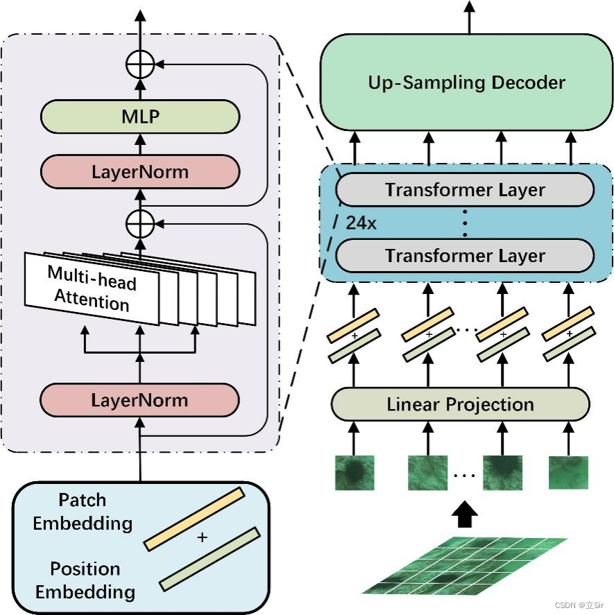
将 Transformer 用于图像分类任务主要有以下 5 个过程：（1）将输入图像或特征进行序列化；（2）添加位置编码；（3）添加可学习的嵌入向量；（4）输入到编码器中进行编码；（5）将输出的可学习嵌入向量用于分类。结构图如下：

2. Patch Embedding

以 b*224*224*3 的输入图片为例。首先进行图像分块，将原图片切分为 14*14 个图像块（Patch），每个 Patch 的大小为 16*16，通过提取输入图片中的平坦像素向量，将每个输入 Patch 送入线性投影层，得到 Patch Embeddings。

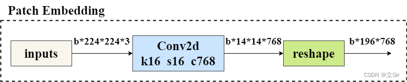
在代码中，先经过一个 kernel=(16,16)，strides=16 的卷积层划分图像块，再将 h和w 维度整合为 num_patches 维度，代表一共有 196 个 patch，每个 patch 为 16*16

# --------------------------------------------- #
# （1）Embedding 层
# inputs代表输入图像，shape为224*224*3
# out_channel代表该模块的输出通道数，即第一个卷积层输出通道数=768
# patch_size代表卷积核在图像上每16*16个区域卷积得出一个值
# --------------------------------------------- #
def patch_embed(inputs, out_channel, patch_size=16):

    # 获得输入图像的shape=[b,224,224,3]
    b, h, w, c = inputs.shape

    # 获得划分后每张图像的size=(14,14)
    grid_h, grid_w = h//patch_size, w//patch_size

    # 计算图像宽高共有多少个像素点 n = h*w
    num_patches = grid_h * grid_w

    # 卷积 [b,224,224,3]==>[b,14,14,768]
    x = layers.Conv2D(filters=out_channel, kernel_size=(16,16), strides=16, padding='same')(inputs)

    # 维度调整 [b,h,w,c]==>[b,n,c]
    # [b,14,14,768]==>[b,196,768]
    x = tf.reshape(x, shape=[b, num_patches, out_channel])

    return x

3. 添加类别标签和位置编码

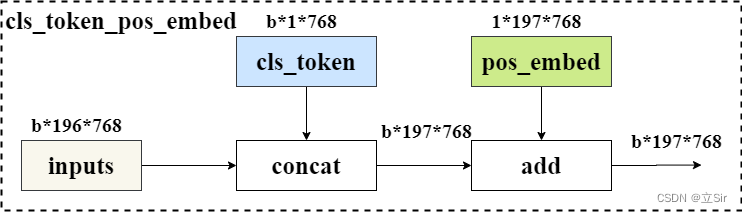
为了输出融合了全局语义信息的向量表示，在第一个输入向量前添加可学习分类变量。经过编码器编码后，在最后一层输出中，该位置对应的输出向量就可以用于分类任务。与其他位置对应的输出向量相比，该向量可以更好的融合图像中各个图像块之间的依赖关系。

在 Transformer 更新的过程中，输入序列的顺序信息会丢失。Transformer 本身并没有办法学习这个信息，所以需要一种方法将位置表示聚合到模型的输入嵌入中。我们对每个 Patch 进行位置编码，该位置编码采用随机初始化，之后参与模型训练。与传统三角函数的位置编码方法不同，该方法是可学习的。

最后，将 Patch-Embeddings 和 class-token 进行堆叠，和 Position-Embeddings 进行叠加，得到最终嵌入向量，该向量输入给 Transformer 层进行后续处理。

扫描二维码关注公众号，回复： 14175800 查看本文章

代码如下：

# --------------------------------------------- #
# （2）类别标签和位置编码
# --------------------------------------------- #
def class_pos_add(inputs):

    # 获得输入特征图的shape=[b,196,768]
    b, num_patches, channel = inputs.shape

    # 类别信息 [1,1,768]
    # 直接通过classtoken来判断类别，classtoken能够学到其他token中的分类相关的信息
    cls_token = layers.Layer().add_weight(name='classtoken', shape=[1,1,channel], dtype=tf.float32,
                                          initializer=keras.initializers.Zeros(), trainable=True)  

    # 可学习的位置变量 [1,197,768], 初始化为0，trainable=True代表可以通过反向传播更新权重
    pos_embed = layers.Layer().add_weight(name='posembed', shape=[1,num_patches+1,channel], dtype=tf.float32,
                                          initializer=keras.initializers.RandomNormal(stddev=0.02), trainable=True)

    # 将类别信息在维度上广播 [1,1,768]==>[b,1,768]
    cls_token = tf.broadcast_to(cls_token, shape=[b, 1, channel])

    # 在num_patches维度上堆叠，注意要把cls_token放前面
    # [b,1,768]+[b,196,768]==>[b,197,768]
    x = layers.concatenate([cls_token, inputs], axis=1)

    # 将位置信息叠加上去
    x = tf.add(x, pos_embed)

    return x  # [b,197,768]

4. 多头自注意力模块

Transformer 层中，主要包含多头注意力机制和多层感知机模块，下面先介绍多头自注意力模块。

单个的注意力机制，其每个输入包含三个不同的向量，分别为 Query向量（Q），Key向量（K），Value向量（V）。他们的结果分别由输入特征图和三个权重做矩阵乘法得到。

$q=X*W^{q} \;\;\;\;\;\ k=X*W^{k} \;\;\;\;\;\ v=X*W^{v}$

接着为每一个输入计算一个得分 $Score = q*k$

为了使梯度稳定，对 Score 的值进行归一化处理，并将结果通过 softmax 函数进行映射。之后再和 v 做矩阵相乘，得到加权后每个输入向量的得分 v。计算完后再乘以一个权重张量 W 提取特征。

计算公式如下，其中 $\sqrt{d_{k}$ 代表 K 向量维度的平方根

$attention = Softmax(\frac{Q*K^{T}}{\sqrt{d_{k}}}*V)$

代码如下：

# --------------------------------------------- #
# （3）多头自注意力模块
# inputs： 代表编码后的特征图
# num_heads: 代表多头注意力中heads个数
# qkv_bias: 计算qkv是否使用偏置
# atten_drop_rate, proj_drop_rate：代表两个全连接层后面的dropout层
# --------------------------------------------- #
def attention(inputs, num_heads, qkv_bias=False, atten_drop_rate=0., proj_drop_rate=0.):

    # 获取输入特征图的shape=[b,197,768]
    b, num_patches, channel = inputs.shape
    # 计算每个head的通道数
    head_channel = channel // num_heads
    # 公式的分母，根号d
    scale = head_channel ** 0.5

    # 经过一个全连接层计算qkv [b,197,768]==>[b,197,768*3]
    qkv = layers.Dense(channel*3, use_bias=qkv_bias)(inputs)
    # 调整维度 [b,197,768*3]==>[b,197,3,num_heads,c//num_heads]
    qkv = tf.reshape(qkv, shape=[b, num_patches, 3, num_heads, channel//num_heads])
    # 维度重排 [b,197,3,num_heads,c//num_heads]==>[3,b,num_heads,197,c//num_heads]
    qkv = tf.transpose(qkv, perm=[2, 0, 3, 1, 4])
    # 获取q、k、v的值==>[b,num_heads,197,c//num_heads]
    q, k, v = qkv[0], qkv[1], qkv[2]

    # 矩阵乘法, q 乘 k 的转置，除以缩放因子。矩阵相乘计算最后两个维度
    # [b,num_heads,197,c//num_heads] * [b,num_heads,c//num_heads,197] ==> [b,num_heads,197,197]
    atten = tf.matmul(a=q, b=k, transpose_b=True) / scale
    # 对每张特征图进行softmax函数
    atten = tf.nn.softmax(atten, axis=-1)
    # 经过dropout层
    atten = layers.Dropout(rate=atten_drop_rate)(atten)
    # 再进行矩阵相乘==>[b,num_heads,197,c//num_heads]
    atten = tf.matmul(a=atten, b=v)

    # 维度重排==>[b,197,num_heads,c//num_heads]
    x = tf.transpose(atten, perm=[0, 2, 1, 3])
    # 维度调整==>[b,197,c]==[b,197,768]
    x = tf.reshape(x, shape=[b, num_patches, channel])

    # 调整之后再经过一个全连接层提取特征==>[b,197,768]
    x = layers.Dense(channel)(x)
    # 经过dropout
    x = layers.Dropout(rate=proj_drop_rate)(x)

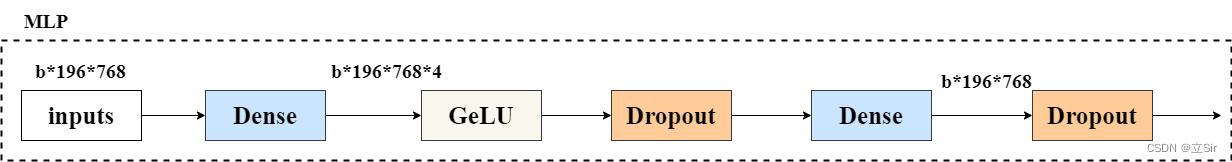
    return x

5. MLP 多层感知器

这个部分简单来看就是两个全连接层提取特征，流程图如下。第一个全连接层通道上升4倍，第二个全连接层通道下降为原来。

代码如下：

# ------------------------------------------------------ #
# （4）MLP block
# inputs代表输入特征图；mlp_ratio代表第一个全连接层上升通道倍数；
# drop_rate代表杀死神经元概率
# ------------------------------------------------------ #
def mlp_block(inputs, mlp_ratio=4.0, drop_rate=0.):

    # 获取输入图像的shape=[b,197,768]
    b, num_patches, channel = inputs.shape

    # 第一个全连接上升通道数==>[b,197,768*4]
    x = layers.Dense(int(channel*mlp_ratio))(inputs)
    # GeLU激活函数
    x = layers.Activation('gelu')(x)
    # dropout层
    x = layers.Dropout(rate=drop_rate)(x)

    # 第二个全连接层恢复通道数==>[b,197,768]
    x = layers.Dense(channel)(x)
    # dropout层
    x = layers.Dropout(rate=drop_rate)(x)

    return x

6. 特征提取模块

Transformer 的单个特征提取模块是由 多头注意力机制 和 多层感知机模块 组合而成，encoder_block 模块的流程图如下。

输入图像像经过 LayerNormalization 标准化后，再经过我们上面定义的多头注意力模块，将输出结果和输入特征图残差连接，图像在特征提取过程中shape保持不变。

将输出结果再经过标准化，然后送入多层感知器提取特征，再使用残差连接输入和输出。

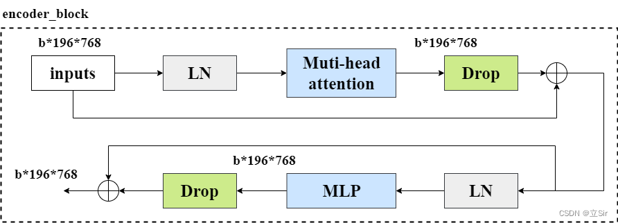
而 transformer 的特征提取模块是由多个 encoder_block 叠加而成，这里连续使用12个 encoder_block 模块来提取特征。

代码如下：

# ------------------------------------------------------ #
# （5）单个特征提取模块
# num_heads：代表自注意力的heads个数
# epsilon：小浮点数添加到方差中以避免除以零
# drop_rate：自注意力模块之后的dropout概率
# ------------------------------------------------------ #
def encoder_block(inputs, num_heads, epsilon=1e-6, drop_rate=0.):

    # LayerNormalization
    x = layers.LayerNormalization(epsilon=epsilon)(inputs)
    # 自注意力模块
    x = attention(x, num_heads=num_heads)
    # dropout层
    x = layers.Dropout(rate=drop_rate)(x)
    # 残差连接输入和输出
    # x1 = x + inputs
    x1 = layers.add([x, inputs])
    
    # LayerNormalization
    x = layers.LayerNormalization(epsilon=epsilon)(x1)
    # MLP模块
    x = mlp_block(x)
    # dropout层
    x = layers.Dropout(rate=drop_rate)(x)
    # 残差连接
    # x2 = x + x1
    x2 = layers.add([x, x1])

    return x2  # [b,197,768]

# ------------------------------------------------------ #
# （6）连续12个特征提取模块
# ------------------------------------------------------ #
def transformer_block(x, num_heads):

    # 重复堆叠12次
    for _ in range(12):
        # 本次的特征提取块的输出是下一次的输入
        x = encoder_block(x, num_heads=num_heads)

    return x  # 返回特征提取12次后的特征图

7. 主干网络

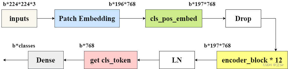
接下来就搭建网络了，将上面所有的模块组合到一起，如下图所示。

在下面代码中要注意的是 cls_ticks = x[:,0] 取出所有的类别标签。因为在 cls_pos_embed 模块中，我们将 cls_token 和输入图像在 patch 维度上堆叠 layers.concate，用于学习每张特征图的类别信息，取出的类别标签 cls_ticks 的 shape 为 [b, 768]。最后经过一个全连接层得出每张图片属于每个类别的得分。

代码如下：

# ---------------------------------------------------------- # 
# （7）主干网络
# batch_shape：代表输入图像的shape=[8,224,224,3]
# classes：代表最终的分类数
# drop_rate：代表位置编码后的dropout层的drop率
# num_heads：代表自注意力机制的heads个数
# epsilon：小浮点数添加到方差中以避免除以零
# ---------------------------------------------------------- # 
def VIT(batch_shape, classes, drop_rate=0., num_heads=12, epsilon=1e-6):

    # 构造输入层 [b,224,224,3]
    inputs = keras.Input(batch_shape=batch_shape)

    # PatchEmbedding层==>[b,196,768]
    x = patch_embed(inputs, out_channel=768)

    # 类别和位置编码==>[b,197,768]
    x = class_pos_add(x)

    # dropout层
    x = layers.Dropout(rate=drop_rate)(x)

    # 经过12次特征提取==>[b,197,768]
    x = transformer_block(x, num_heads=num_heads)

    # LayerNormalization
    x = layers.LayerNormalization(epsilon=epsilon)(x)

    # 取出特征图的类别标签，在第（2）步中我们把类别标签放在了最前面
    cls_ticks = x[:,0]
    # 全连接层分类
    outputs = layers.Dense(classes)(cls_ticks)

    # 构建模型
    model = keras.Model(inputs, outputs)

    return model

8. 查看模型结构

这里有个注意点，keras.Input() 的参数问题，创建输入层时，参数 shape 不需要指定batch维度，batch_shape 需要指定batch维度。

keras.Input(shape=None, batch_shape=None, name=None, dtype=K.floatx(), sparse=False, tensor=None)
'''
shape: 形状元组（整型），不包括batch size。for instance, shape=(32,) 表示了预期的输入将是一批32维的向量。
batch_shape: 形状元组（整型），包括了batch size。for instance, batch_shape=(10,32)表示了预期的输入将是10个32维向量的批次。
'''

接收模型后，通过 model.summary() 查看模型结构和参数量，通过 get_flops() 参看浮点计算量。

# ---------------------------------------------------------- # 
# （8）接收模型
# ---------------------------------------------------------- # 
if __name__ == '__main__':

    batch_shape = [8,224,224,3]  # 输入图像的尺寸
    classes = 1000  # 分类数

    # 接收模型
    model = VIT(batch_shape, classes)

    # 查看模型结构
    model.summary()
    
    # 查看浮点计算量 flops = 51955425272
    from keras_flops import get_flops
    print('flops:', get_flops(model, batch_size=8))

参数量和计算量如下

----------------------------------------------------------------
add_84 (Add)                   (8, 197, 768)        0           ['dropout_368[0][0]',            
                                                                  'add_83[0][0]']                 
                                                                                                  
 layer_normalization_126 (Layer  (8, 197, 768)       1536        ['add_84[0][0]']                 
 Normalization)                                                                                   
                                                                                                  
 tf.__operators__.getitem_187 (  (8, 768)            0           ['layer_normalization_126[0][0]']
 SlicingOpLambda)                                                                                 
                                                                                                  
 dense_246 (Dense)              (8, 1000)            769000      ['tf.__operators__.getitem_187[0]
                                                                 [0]']                            

==============================================================
Total params: 86,387,944
Trainable params: 86,387,944
Non-trainable params: 0
flops: 51955425272
______________________________________________________________

【神经网络】(21) Vision Transformer 代码复现，网络解析，附TensorFlow完整代码

1. 引言

2. Patch Embedding

3. 添加类别标签和位置编码

4. 多头自注意力模块

5. MLP 多层感知器

6. 特征提取模块

7. 主干网络

8. 查看模型结构

猜你喜欢