支持向量机SVM 原理、推导与Matlab实现

1 内容

本文首先介绍SVM的原理，随后给出SVM的公式推导、并使用Matlab的二次规划函数进行求解。

2 SVM原理

我们前面学过了线性回归和线性分类器。我们来回顾一下。

2.1 线性回归

线性回归试图找到一条线，让每个点在Y方向上离线越接近越好。就是说，每个数据点做一条垂直的线相较于回归直线，这些线段（图中红色线段）的长度的平方和最小就是要最优化的函数。如图。

$$J(w,b) = \sum_i (w^Tx_i+b - y_i)^2$$
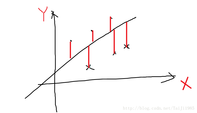
我们要找到一个合适的w和b使得$J(w,b)最小。

$$\min_{w,b} J(w,b)$$

2.2 线性分类器

再回顾一下线性分类器。设有数据集$D=\{ x_i ,y_i \}_{i=1}^N, y_i \in \{-1,1\}$, $x_i$ 为K维列向量， 即$x \in R^{K\times1}$。$y_i$表示$x_i$所属的类，其取值为1和-1。

我们的目标是想找出一条线$y = w^Tx+b$,使得对于所有的$x_i$ 都有

$$y_i(w^Tx_i+b) > 0$$

扫描二维码关注公众号，回复： 138453 查看本文章

这个公式的意义在于， 当y_i为1的时候， $w^Tx_i+b$ 要求为正数，这样他们的成绩为正，当$y_i$为-1时，$w^Tx_i+b$ 要求为负数，这样乘积仍然为正。

找到这样一组w和b后，将新的数据x带入$w^Tx+b$如果结果为正，则属于1类，结果为负，属于-1类。就完成了分类。

2.3 SVM

满足线性分类器条件的线有很多种，那么哪一种是最好的呢？ 我们应当如何评价一个线是好还是坏呢？

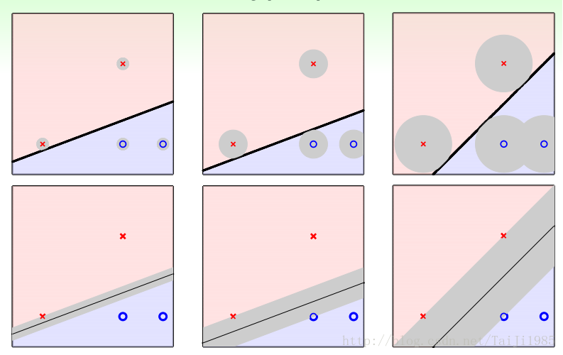
上图中给出了同一组数据的三种划分方式。每一种划分方式都可以达到100%的分类准确率。但他们应对误差的能力是不同的。在实际问题中，采集数据是有误差的。那么哪一个划分方法能更好的应对误差呢？ 可以看到是第三组图。第三组图有什么特征呢？ 分割带最胖！

我们如何用数学来描述“分隔带最胖”这个说法？ 每个点都与分割线（或者分割平面）有一个距离。所有点中距离的最小值如果最大，那么这就是分隔带最胖。在图三中，两个x和一个o是距离分割线最近的，他们距离分割线最远，那么这个分割线就是最优的分割线。

这个选取“最胖”的线作为分割线（分割面）的方法就是支持向量机。

3 公式推导

3.1 点到直线的距离

设有$x'$和$x''$位于 分割线（推广到多维称 超平面）上，则满足分割线的公式，即

$$w^Tx' +b = 0$$
$$w^Tx'' +b = 0$$

两式相减，得到

$$w^T(x' - x'') = 0$$
因为x’和x”都是超平面上的点，那么x’-x”这个向量就是超平面上的向量。 这个向量与w^T的内积为0，说明w和x’-x” 相互垂直， $w$为超平面的法向量。

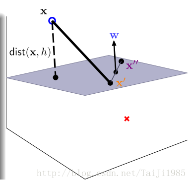
任意一点x到平面的距离 就是 x-x’这个向量在w方向上的投影的长度。如图

$$dist(x,h) = | \frac{w^T}{||w||} (x-x') | = \frac{|w^Tx+b|}{||w||}$$

对于可以正确分类的超平面，都满足线性分类器的条件，即

$$y_i(w^Tx_i+b) > 0$$

那么就可以去掉上述公式中的绝对值。

$$dist(x_i,h) =\frac{y_i(w^Tx_i+b)}{||w||}$$

上述“最胖”的概念就可以用下面的公式表示

$$\max_{b,w} = margin(b,w) \\ \text{使得, 所有的} y_i(w^Tx_i+b)>0 \text{且} margin(b,w) = \min_{i=1,...N} dist(x_i,h)$$

假定距离超平面最近的点为$x_i$， 令 $t = y_i(w^Tx+b)$ 。 将w和b同时除以t就可以得到新的w和b。
有 $1 = y_i(w^Tx+b)$ 。 注意，因为我们要找到最小的 $dist(x_i,h)$，对w和b 的放缩不会影响谁是最近的点这个结果。也不会影响超平面的位置因为
$w^Tx+b=0$和 $(w^Tx/t+b/t) = 0$并无分别。

所以，不失一般性，可以认为对于距离最近的点$w^Tx_i+b = 1$,其他点距离都比这个大，那么就有

$$y_i(w^Tx_i+b) >= 1$$

上述条件中，$margin(b,w) = \min_{i=1,...N} dist(x_i,h)$不方便计算，可以用上面的不等式来表示。

另外， $margin(b,w)$ 表示的是最近的点到平面的距离，因为$w^Tx_i+b = 1$，所以

$$margin(b,w) = \frac{1}{ ||w|| }$$

这样我们就得到了

$$\max_{b,w} \frac{1}{||w||} ，使得 y_i(w^Tx_i+b) >= 1$$

我们不喜欢$\max$，喜欢min,所以把求一个倒数。 一个正数取最大值时，其倒数取最小值。

$$\min_{b,w} ||w|| ，使得 y_i(w^Tx_i+b) >= 1$$
这个 $||w||$，可以用 $w^Tw$ 开方 得到。开方不影响大小关系，所以我们不开方，并加上一个系数，就得到了

$$\min_{b,w} \frac{1}{2}w^Tw ，使得 y_i(w^Tx_i+b) >= 1$$

这个东西就是一个二次规划问题，我们就可以用二次规划工具求解了。

转化为二次规划的标准型

二次规划的标准型为以下形式

$$优化 u \leftarrow QP(H,f,A,b) \\ \min_u \frac{1}{2}u^THu+f^Tu , \\ 满足 a_m^Tu <= b_m$$

将SVM公式，转化为上述形式，令u为w的增广形式

$$u = \begin{bmatrix} b \\ w \end{bmatrix}$$

$$H = \begin{bmatrix} 0 & 0_K \\ 0_K & I_K \end{bmatrix}$$ , K为w的维度，H是(K+1)*(K+1)的矩阵，除了（1，1）点，其他对角线均为1

举个例子

H = [
  0 0 0 ;
  0 1 0 ;
  0 0 1
]

这样$u^THu$就能凑出 $w^Tw$ 这个结果。
令

$$f = 0_K \in R^{K\times1}$$
让一次项为0。

$y_i(w^Tx_i+b) >= 1$修改为 $-y_i(w^Tx_i+b) <= -1$

$A_i = - y_i [ 1 , x_i]$ , 使得$b_i = -1$

matlab的 quadprog

quadprog Quadratic programming.
X = quadprog(H,f,A,b) attempts to solve the quadratic programming
problem:

         min 0.5*x'*H*x + f'*x   subject to:  A*x <= b 
          x    

X = quadprog(H,f,A,b,Aeq,beq) solves the problem above while 
additionally satisfying the equality constraints Aeq*x = beq.

X = quadprog(H,f,A,b,Aeq,beq,LB,UB) defines a set of lower and upper
bounds on the design variables, X, so that the solution is in the 
range LB <= X <= UB. Use empty matrices for LB and UB if no bounds 
exist. Set LB(i) = -Inf if X(i) is unbounded below; set UB(i) = Inf if 
X(i) is unbounded above.

X = quadprog(H,f,A,b,Aeq,beq,LB,UB,X0) sets the starting point to X0.

X = quadprog(H,f,A,b,Aeq,beq,LB,UB,X0,OPTIONS) minimizes with the 
default optimization parameters replaced by values in the structure 
OPTIONS, an argument created with the OPTIMSET function. See OPTIMSET 
for details. 

X = quadprog(PROBLEM) finds the minimum for PROBLEM. PROBLEM is a
structure with matrix 'H' in PROBLEM.H, the vector 'f' in PROBLEM.f,
the linear inequality constraints in PROBLEM.Aineq and PROBLEM.bineq,
the linear equality constraints in PROBLEM.Aeq and PROBLEM.beq, the
lower bounds in PROBLEM.lb, the upper bounds in PROBLEM.ub, the start
point in PROBLEM.x0, the options structure in PROBLEM.options, and 
solver name 'quadprog' in PROBLEM.solver. Use this syntax to solve at 
the command line a problem exported from OPTIMTOOL. The structure 
PROBLEM must have all the fields. 

[X,FVAL] = quadprog(H,f,A,b) returns the value of the objective 
function at X: FVAL = 0.5*X'*H*X + f'*X.

[X,FVAL,EXITFLAG] = quadprog(H,f,A,b) returns an EXITFLAG that 
describes the exit condition of quadprog. Possible values of EXITFLAG 
and the corresponding exit conditions are

All algorithms:
  1  First order optimality conditions satisfied.
  0  Maximum number of iterations exceeded.
 -2  No feasible point found.
 -3  Problem is unbounded.
Interior-point-convex only:
 -6  Non-convex problem detected.
Trust-region-reflective only:
  3  Change in objective function too small.
 -4  Current search direction is not a descent direction; no further 
      progress can be made.
Active-set only:
  4  Local minimizer found.
 -7  Magnitude of search direction became too small; no further 
      progress can be made. The problem is ill-posed or badly 
      conditioned.

[X,FVAL,EXITFLAG,OUTPUT] = quadprog(H,f,A,b) returns a structure
OUTPUT with the number of iterations taken in OUTPUT.iterations,
maximum of constraint violations in OUTPUT.constrviolation, the 
type of algorithm used in OUTPUT.algorithm, the number of conjugate
gradient iterations (if used) in OUTPUT.cgiterations, a measure of 
first order optimality (large-scale algorithm only) in 
OUTPUT.firstorderopt, and the exit message in OUTPUT.message.

[X,FVAL,EXITFLAG,OUTPUT,LAMBDA] = quadprog(H,f,A,b) returns the set of 
Lagrangian multipliers LAMBDA, at the solution: LAMBDA.ineqlin for the 
linear inequalities A, LAMBDA.eqlin for the linear equalities Aeq, 
LAMBDA.lower for LB, and LAMBDA.upper for UB.

See also linprog, lsqlin.

Reference page in Help browser
   doc quadprog

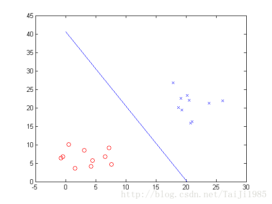
matlab求解SVM

function test_svm()
t1  = 5+4*randn(2,10);
t2 = 20+4*randn(2,10);
X = [t1 t2]
X = [t1 t2];
Y = [ones(10,1) ; -ones(10,1)]

plot(t1(1,:),t1(2,:),'ro');
hold on;
plot(t2(1,:),t2(2,:),'bx');
u = svm(X,Y)
x = [-u(1)/u(2) , 0];
y = [0 , -u(1)/u(3)];
plot(x,y);

end

function u = svm( X,Y )
%SVM Summary of this function goes here
%   Detailed explanation goes here
    [K,N] = size(X);
    u0= rand(K+1,1); %  u= [b ; w];
    A = - repmat(Y,1,K+1).*[ones(N,1) X'];
    b = -ones(N,1);

    H = eye(K);
    H = [zeros(1,K);H];
    H = [zeros(K+1,1) H];

    p = zeros(K+1,1);
    lb = -10*ones(K+1,1);
    rb = 10*ones(K+1,1);

    options = optimset;    % Options是用来控制算法的选项参数的向量
    options.LargeScale = 'off';
    options.Display = 'off';
    options.Algorithm = 'active-set';

    [u,val] = quadprog(H,p,A,b,[],[],lb,rb,u0,options)
end

ans =

   -0.7964    6.3340
    6.5654    6.8067
    4.4789    5.7348
    3.0954    8.4481
   -0.4468    6.8201
    1.6052    3.6605
    7.2111    9.1564
    0.5294   10.0426
    7.6406    4.7285
    4.2191    4.1296
   18.7876   20.0922
   20.2052   23.3043
   26.1079   21.8677
   19.1611   22.5008
   20.7329   15.8809
   23.7969   21.2282
   20.5407   22.0610
   21.0456   16.2341
   19.3506   19.4158
   17.8720   26.7284


Y =

     1
     1
     1
     1
     1
     1
     1
     1
     1
     1
    -1
    -1
    -1
    -1
    -1
    -1
    -1
    -1
    -1
    -1

Optimization terminated.

u =

    2.3951
   -0.1186
   -0.0590


val =

    0.0088

感想

这个程序看起来非常的简单，但也调试了好久，主要是当时 $y_i(w^Tx_i+b) >= 1$ ,两边乘以 -1时，忘了将右侧改为1 ，导致，w的值永远是0 。但因为平时用二次优化比较少，一直怀疑是不是这个最优化函数运行不正常。。。。 这就影响了正常调错。。。

不足

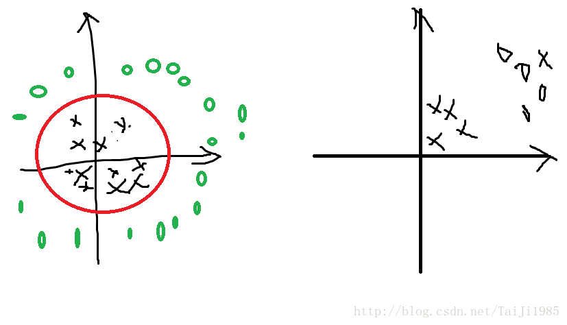
其一、 这是一个线性分类器，对于线性不可分的情况不能解决。那么怎么办呢？ 将当前的x，通过一个函数映射到其他空间，使得在新的空间线性可分。如上图左，使用一个圆可以很简单的将黑色的×和红色的圈分隔开，但圆不是线性的。样本 $x= [ x_1,x_2]$ ,$x_1,x_2$ 分别为横坐标和纵坐标。 那么令 $u = x_1^2 + x_2^2 = x^Tx$ ， 就可以讲这个线性不可分的问题变成线性可分。

其二、这个分类器不允许有错误，要求必须每一个数据都分对，如果找不到这样的线，那么就不能得到正确的解。 实际问题中，常常因为数据采集误差，或者模型本身问题而无法达到所有数据都正确分类的结果。如右图中，有一个×在右上角，不论选取何种曲线，都无法将其线性分类，所以最好的办法就是对少量错误视而不见。这时候就需要一个软分隔的SVM，它应能容忍少量的错误。

这两个问题都会在后续的博客中解释。