论文
https://www.pnas.org/content/118/20/e2010588118
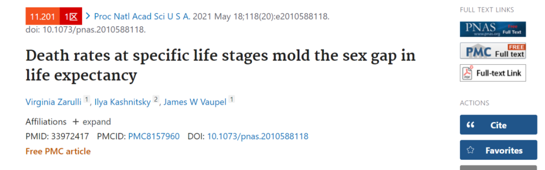
Death rates at specific life stages mold the sex gap in life expectancy
论文本地存储 e2010588118.full.pdf
很有意思的一篇论文,研究的内容是为什么女生比男生活的时间长(Why do women live longer than men?)哈哈哈。但是整篇论文我还没有看明白,所以先不给大家介绍结论了。
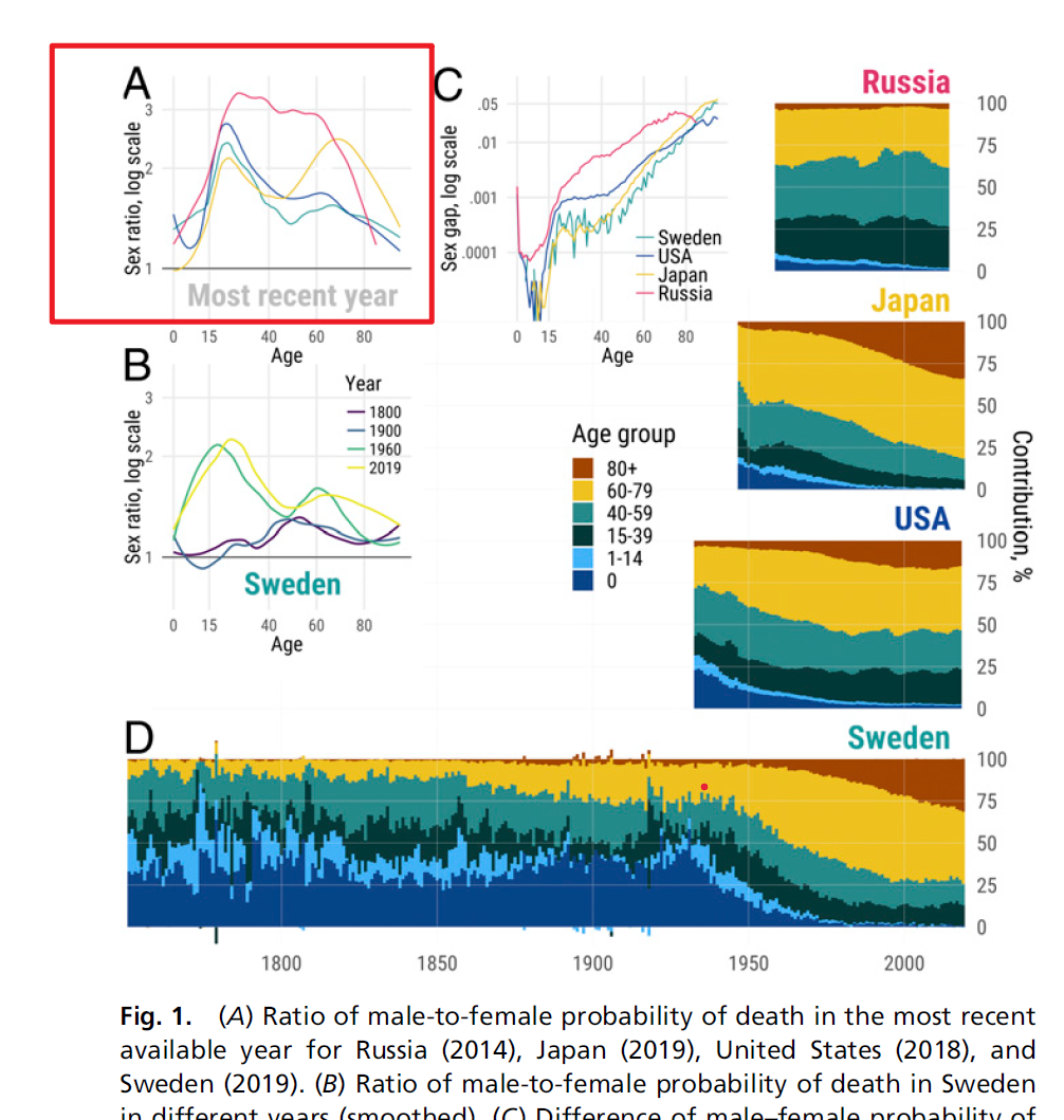
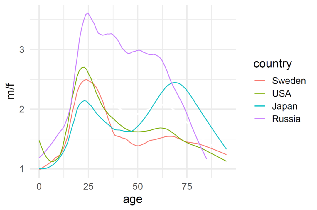
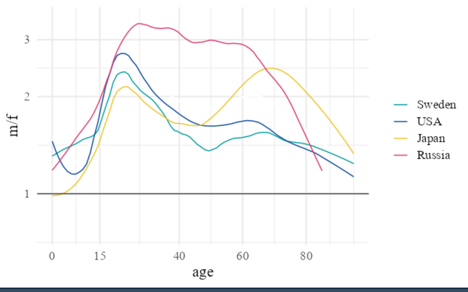
这篇论文的数据和代码是公开的,链接是 https://github.com/CPop-SDU/sex-gap-e0-pnas,我们按照他提供的代码和数据试着复原一下论文里的图。今天的推文重复的内容是论文中的Figure1A
分组折线图
用到的数据集是链接里的dat文件夹下的 df4qx.rda文件,
首选是导入数据
load("data/df4qx.rda")
head(df4qx)
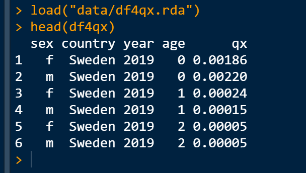
这个是一个长格式数据,把它转变成宽格式
#install.packages("tidyverse")
library(tidyverse)
df4qx %>%
  pivot_wider(names_from = sex,values_from = qx) %>%
  head()
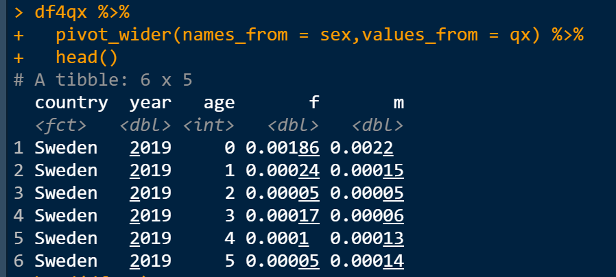
这一步是为了方便计算不同年龄男女死亡率的比例
ggplot2作图
df4qx %>%
  pivot_wider(names_from = sex,values_from = qx) -> dftemp
最基本的图
library(ggplot2)
dftemp %>%
  ggplot(aes(age,y=m/f,color=country))+
  geom_smooth(se=F,size=1,color="#ffffff",span=0.25)+
  geom_smooth(se = F, size = .5, span = .25)+
  theme_minimal(base_size = 16)
这里原始代码还设置字体了,我这里就跳过了,因为我的电脑没有这个字体
接下来做细节调整
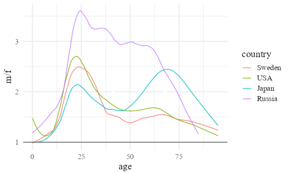
添加一条水平辅助线
dftemp %>%
  ggplot(aes(age,y=m/f,color=country))+
  geom_smooth(se=F,size=1,color="#ffffff",span=0.25)+
  geom_smooth(se = F, size = .5, span = .25)+
  theme_minimal(base_size = 16,base_family = "serif")+
  geom_hline(yintercept = 1, color = "gray25",  size = .5)
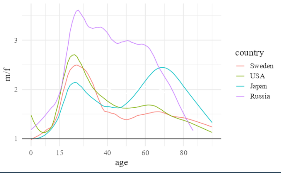
更改x轴刻度范围
dftemp %>%
  ggplot(aes(age,y=m/f,color=country))+
  geom_smooth(se=F,size=1,color="#ffffff",span=0.25)+
  geom_smooth(se = F, size = .5, span = .25)+
  theme_minimal(base_size = 16,base_family = "serif")+
  geom_hline(yintercept = 1, color = "gray25",  size = .5)+
  scale_x_continuous(breaks = c(0, 15, 40, 60, 80))
对y轴进行log2转换
dftemp %>%
  ggplot(aes(age,y=m/f,color=country))+
  geom_smooth(se=F,size=1,color="#ffffff",span=0.25)+
  geom_smooth(se = F, size = .5, span = .25)+
  theme_minimal(base_size = 16,base_family = "serif")+
  geom_hline(yintercept = 1, color = "gray25",  size = .5)+
  scale_x_continuous(breaks = c(0, 15, 40, 60, 80))+
  scale_y_continuous(
  trans = "log",
  breaks = c(.5, 1, 2, 3),
  labels = c("", 1, 2, 3),
  limits = c(.75, 3.5))
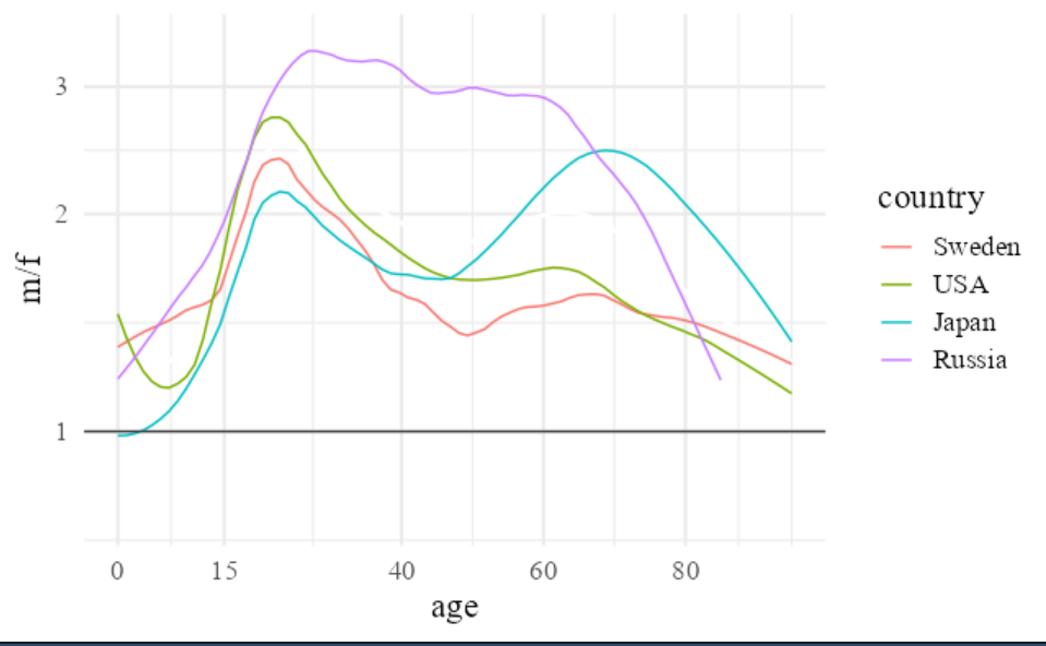
这一步为啥要做转化呢 有些没看明白
自定义配色
pal_safe_five <- c(
  "#eec21f", # default R 4.0 yellow
  "#009C9C", # light shade of teal: no red, equal green and blue
  "#df356b", # default R 4.0 red
  "#08479A", # blues9[8] "#08519C" made a bit darker
  "#003737" # very dark shade of teal
)

pal_safe_five_ordered <- pal_safe_five[c(5,2,1,3,4)]
pal_four <- pal_safe_five_ordered[c(2,5,3,4)]

dftemp %>%
  ggplot(aes(age,y=m/f,color=country))+
  geom_smooth(se=F,size=1,color="#ffffff",span=0.25)+
  geom_smooth(se = F, size = .5, span = .25)+
  theme_minimal(base_size = 16,base_family = "serif")+
  geom_hline(yintercept = 1, color = "gray25",  size = .5)+
  scale_x_continuous(breaks = c(0, 15, 40, 60, 80))+
  scale_y_continuous(
    trans = "log",
    breaks = c(.5, 1, 2, 3),
    labels = c("", 1, 2, 3),
    limits = c(.75, 3.5))+
  scale_color_manual(NULL, values = pal_four)
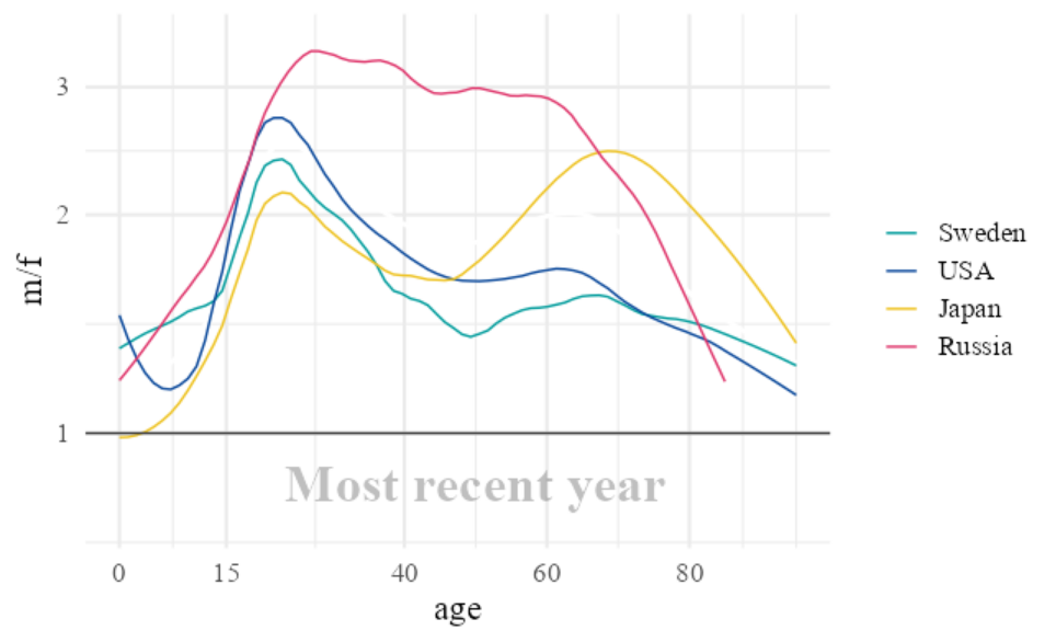
添加文本注释
dftemp %>%
  ggplot(aes(age,y=m/f,color=country))+
  geom_smooth(se=F,size=1,color="#ffffff",span=0.25)+
  geom_smooth(se = F, size = .5, span = .25)+
  theme_minimal(base_size = 16,base_family = "serif")+
  geom_hline(yintercept = 1, color = "gray25",  size = .5)+
  scale_x_continuous(breaks = c(0, 15, 40, 60, 80))+
  scale_y_continuous(
    trans = "log",
    breaks = c(.5, 1, 2, 3),
    labels = c("", 1, 2, 3),
    limits = c(.75, 3.5))+
  scale_color_manual(NULL, values = pal_four)+
  annotate(
    "text", x = 50, y = .9,
    label = "Most recent year",
    size = 8.5, color = "grey50", alpha = .5,
    vjust = 1, family = "serif", fontface = 2
  )
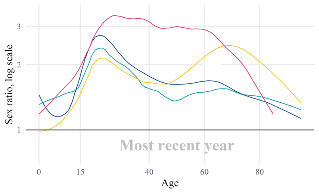
去掉图例并更改坐标轴标题
dftemp %>%
  ggplot(aes(age,y=m/f,color=country))+
  geom_smooth(se=F,size=1,color="#ffffff",span=0.25)+
  geom_smooth(se = F, size = .5, span = .25)+
  theme_minimal(base_size = 16,base_family = "serif")+
  geom_hline(yintercept = 1, color = "gray25",  size = .5)+
  scale_x_continuous(breaks = c(0, 15, 40, 60, 80))+
  scale_y_continuous(
    trans = "log",
    breaks = c(.5, 1, 2, 3),
    labels = c("", 1, 2, 3),
    limits = c(.75, 3.5))+
  scale_color_manual(NULL, values = pal_four)+
  annotate(
    "text", x = 50, y = .9,
    label = "Most recent year",
    size = 8.5, color = "grey50", alpha = .5,
    vjust = 1, family = "serif", fontface = 2
  )+
  theme(
    legend.position = "none",
    panel.grid.minor = element_blank()
  )+
  labs(
    y = "Sex ratio, log scale",
    x = "Age"
  )
欢迎大家关注我的公众号
小明的数据分析笔记本
今天推文的示例数据和代码可以在公众号后台留言 20210829 获取
(精确匹配开头结尾都不能有空格)
小明的数据分析笔记本 公众号 主要分享:1、R语言和python做数据分析和数据可视化的简单小例子;2、园艺植物相关转录组学、基因组学、群体遗传学文献阅读笔记;3、生物信息学入门学习资料及自己的学习笔记!
后记
今天发现视频号和公众号现在可以带货了,京东和拼多多平台的商品可以生成我自己的链接,如果有人通过这个链接购买商品 我就可以得到相应比例的佣金。比如我今天买了两双鞋,总共花费400多,我拿到的佣金是20几块。大家如果经常在京东或者拼多多买东西的话可以加一下下面的微信群,比如你想买一件东西,可以先把商品的链接发给我,我生成我专属的链接,然后你再通过我的专属链接买,这样我就能有收入,我可以将收入的一半再转给你,你能省几块钱,我也能赚几块钱。

本文分享自微信公众号 - 小明的数据分析笔记本(gh_0c8895f349d3)。
如有侵权,请联系 [email protected] 删除。
本文参与“OSC源创计划”,欢迎正在阅读的你也加入,一起分享。