0引言

在数据可视化——一文入门ggplot2中介绍了ggplot2包以及他的基本语法。在R语言可视化——ggplot2包的八种默认主题及其扩展包中介绍ggplot2包中默认的八种主题。今天实战一下，使用ggplot2包画回归曲线添加回归方程、方差分析表，调整的 $R^2$ 、调整回归数据等，本篇使用默认主题。

1、构造回归数据

画图离不开数据，下面使用生成随机数的方式生成数据，为了代码的可重复性设置随机数种子。

> n = 100
> set.seed(0)
> x <- runif(n, 0, 4)
> y <- x^2 - x + rnorm(n, 0, 0.4)
> MyClass <- factor((x>0) + (x>1) + (x>2) + (x>3),
+ labels = c("0-1", "1-2", "2-3", "3-4"))
> Data <- data.frame(x = x, y = y, class = MyClass)
> head(Data)
          x           y class
1 3.5867888  9.38472004   3-4
2 1.0620347 -0.08479814   1-2
3 1.4884956  1.70366940   1-2
4 2.2914135  2.64102651   2-3
5 3.6328312  9.54268009   3-4
6 0.8067277 -0.05586157   0-1
> str(Data)
'data.frame':   100 obs. of  3 variables:
 $ x    : num  3.59 1.06 1.49 2.29 3.63 ...
 $ y    : num  9.3847 -0.0848 1.7037 2.641 9.5427 ...
 $ class: Factor w/ 4 levels "0-1","1-2","2-3",..: 4 2 2 3 4 1 4 4 3 3 ...
> class(Data)
[1] "data.frame"

下部分使用本节的数据进行画图。

2、画图

2.1载入包

除了载入ggplot2包之外还需要载入扩展包：ggmisc。

library(ggplot2) #加载ggplot2包
library(ggpmisc) #加载ggpmisc包

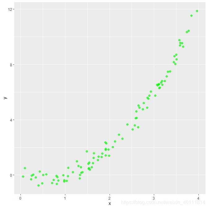
2.2 准备数据添加散点

p <- ggplot(Data, aes(x, y)) +
 geom_point(color = "green",size = 2, alpha = 0.65)
p

在这里插入图片描述

2.3添加回归线

se参数控制是否显示误差区域。

p + 
 stat_smooth(color = "blue", formula = y ~ x, fill = "blue", method = "lm")+
 stat_fit_deviations(formula = y ~ x, color = "skyblue")

在这里插入图片描述

2.5 添加公式R方

注：label.x 、 label.y调整公式位置。

p + 
 stat_smooth(color = "blue", formula = y ~ x,fill = "blue", method = "lm") +
 stat_poly_eq(
   aes(label = paste(..eq.label.., ..adj.rr.label.., sep = '~~~~~~')),
   formula = y ~ x,  parse = TRUE,
     size = 4, # 公式字体大小
     label.x = 0.1,
     label.y = 0.8)

在这里插入图片描述

2.6 添加方差分析表

p + 
 stat_smooth(color = "blue", formula = y ~ x,fill = "blue", method = "glm") +
 stat_poly_eq(
   aes(label = paste(..eq.label.., ..adj.rr.label.., sep = '~~~~~~')),
   formula = y ~ x,  parse = TRUE,
     size = 4, #公式字体大小
     label.x = 0.1,
     label.y = 0.8) + 
 stat_fit_tb(method = "lm",
             method.args = list(formula = y ~ x),
             tb.type = "fit.anova",
             tb.vars = c(Effect = "term",
                         "自由度" = "df",
                         "均方" = "meansq",
                         "italic(F值)" = "statistic",
                         "italic(P值)" = "p.value"),
             label.y = 0.7, label.x = 0.05,
             size = 4.5,
             parse = TRUE
)

在这里插入图片描述

2.6 回归数据调整

模型的参数形式可以通过I函数去调整，如下把一次数据换成二次的数据。

p + 
 stat_smooth(color = "blue", formula = y ~ I(x^2),fill = "blue", method = "glm") +
 stat_poly_eq(
   aes(label = paste(..eq.label.., ..adj.rr.label.., sep = '~~~~~~')),
   formula = y ~ I(x^2),  parse = TRUE,
     size = 4, #公式字体大小
     label.x = 0.1,
     label.y = 0.8) + 
 stat_fit_tb(method = "lm",
             method.args = list(formula = y ~ I(x^2)),
             tb.type = "fit.anova",
             tb.vars = c(Effect = "term",
                         "自由度" = "df",
                         "均方" = "meansq",
                         "italic(F值)" = "statistic",
                         "italic(P值)" = "p.value"),
             label.y = 0.7, label.x = 0.05,
             size = 4.5,
             parse = TRUE
)

在这里插入图片描述
上面可以看出 $R^2$ 和回归的效果变得更好了。