TensorFlow2.0 模型构建

模型构建

# -*- coding: utf-8 -*-
# @Time    : 2021/7/12 8:36
# @Author  : 
import matplotlib.pyplot as plt
import pandas as pd
import tensorflow as tf

fashion_mnist = tf.keras.datasets.fashion_mnist
(x_train_all, y_train_all), (x_test, y_test) = fashion_mnist.load_data()

# 训练集拆分为训练集和验证集
x_valid, x_train = x_train_all[:5000], x_train_all[5000:]
y_valid, y_train = y_train_all[:5000], y_train_all[5000:]
print(x_valid.shape, y_valid.shape)
print(x_train.shape, y_train.shape)
print(x_test.shape, y_test.shape)

#### 模型构建
# Sequential把一系列层次堆叠
# tf.keras.models.Sequential()

"""
model = tf.keras.Sequential()
# 输入层
# 将输入图片进行展开,输入是28*28的图像
# Flatten展平 将28*28二维矩阵展平为28*28一维向量
model.add(tf.keras.layers.Flatten(input_shape=[28, 28]))
# 全连接层(神经网络里最普通的一种神经网络,有层次,下一层所有单元和上一层单元都进行一一连接)
# 单元数300 activation激活函数
model.add(tf.keras.layers.Dense(300, activation="relu"))
model.add(tf.keras.layers.Dense(100, activation="relu"))
model.add(tf.keras.layers.Dense(10, activation="softmax"))
"""
# relu: y=max(0,x)
# softmax: 将向量变成概率分布. x = [x1, x2, x3],
#          y=[e^x1/sum, e^x2/sum, e^s3/sum],sum=e^x1 + e^x2 + e^x3

model = tf.keras.Sequential([
    tf.keras.layers.Flatten(input_shape=[28, 28]),
    tf.keras.layers.Dense(300, activation="relu"),
    tf.keras.layers.Dense(100, activation="relu"),
    tf.keras.layers.Dense(10, activation="softmax")
])
# loss损失函数
# reason for sparse: y->index. y->one_hot->[]
# 如果y是数 sparse_categorical_crossentropy
# 如果y是向量categorical_crossentropy
# optimizer模型的求解方法
# metrics 指标
model.compile(loss="sparse_categorical_crossentropy",
              # optimizer="sgd",
              optimizer="adam",
              metrics=["accuracy"])

# 查看模型有多少层
print(model.layers)

# 查看模型概况
print(model.summary())
# 第一层[None,784]:样本数*784的矩阵
# 经过全连接层之后变成[None, 300]:样本数*300的矩阵
# W(矩阵) b(偏置)
# 784*300+300=235500
# [None,784] * W + b -> [None, 300] W.shape [784, 300], b = [300]

# 训练函数
# epochs遍历训练集次数
history = model.fit(x_train, y_train, epochs=10,
                    validation_data=(x_valid, y_valid))

type(history)

# 查看相应数据
print(history.history)


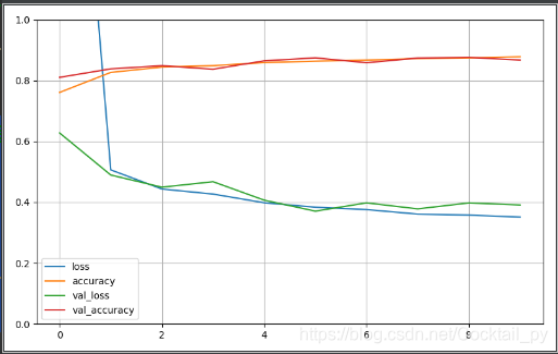
def plot_learning_curves(history):
    pd.DataFrame(history.history).plot(figsize=(8, 5))
    plt.grid(True)
    plt.gca().set_ylim(0, 1)
    plt.show()


plot_learning_curves(history)

2-4实战分类之模型构建