一、numpy
1、读写文件
1>二进制文件读写
import numpy as np
"""
二进制文件、文本文件
"""
arr1 = np.arange(16).reshape(4, 4)
print(arr1)
"""
[[ 0 1 2 3]
[ 4 5 6 7]
[ 8 9 10 11]
[12 13 14 15]]
"""
np.save("arr1", arr1)
arr_new = np.load("arr1.npy")
print(arr_new)
"""
[[ 0 1 2 3]
[ 4 5 6 7]
[ 8 9 10 11]
[12 13 14 15]]
"""
arr2 = np.zeros((2, 2))
np.savez("arr_all", arr1, arr2)
arr_all = np.load("arr_all.npz")
print(arr_all)
for tmp in arr_all:
print(tmp)
2>文本文件读写
np.savetxt("arr1.txt", arr1, fmt="%d", delimiter=",")
np.savetxt("arr1.csv", arr1, fmt="%d", delimiter=",")
res = np.loadtxt("arr1.txt", delimiter=",", dtype=int)
print("res\n", res, type(res))
"""
res
[[ 0 1 2 3]
[ 4 5 6 7]
[ 8 9 10 11]
[12 13 14 15]] <class 'numpy.ndarray'>
"""
2、数组去重
import numpy as np
arr1 = np.array([1, 2, 3, 4, 6, 3, 2, 2, 1])
res = np.unique(arr1)
print("去重后\n", res)
"""
去重后
[1 2 3 4 6]
"""
arr2 = np.array([["A", 1],
[1, 2],
[2, 3],
["A", 1]])
res = np.unique(arr2)
print("去重后\n", res)
"""
去重后
['1' '2' '3' 'A']
"""
res = np.unique(arr2, axis=0)
print("去重后\n", res)
"""
去重后
[['1' '2']
['2' '3']
['A' '1']]
"""
3、数组重复
import numpy as np
"""
重复的两种形式:
repeat
tile
"""
arr = np.arange(9).reshape(3, 3)
print(arr)
"""
[[0 1 2]
[3 4 5]
[6 7 8]]
"""
res = np.repeat(arr, repeats=3)
print("res\n", res)
"""
res
[0 0 0 1 1 1 2 2 2 3 3 3 4 4 4 5 5 5 6 6 6 7 7 7 8 8 8]
"""
res = np.repeat(arr, repeats=3, axis=0)
print("res\n", res)
"""
res
[[0 1 2]
[0 1 2]
[0 1 2]
[3 4 5]
[3 4 5]
[3 4 5]
[6 7 8]
[6 7 8]
[6 7 8]]
"""
res = np.repeat(arr, repeats=3, axis=1)
print("res\n", res)
"""
res
[[0 0 0 1 1 1 2 2 2]
[3 3 3 4 4 4 5 5 5]
[6 6 6 7 7 7 8 8 8]]
"""
res = np.tile(arr, (1, 2))
print("res\n", res)
"""
res
[[0 1 2 0 1 2]
[3 4 5 3 4 5]
[6 7 8 6 7 8]]
"""
4、数组排序
1>一维数组的排序
import numpy as np
arr = np.array([9, 8, 7, 1, 2, 3])
res = np.sort(arr)
print("原始数组", arr)
print("排序后的结果", res)
res = np.argsort(arr)
print("res", res)
new_arr = arr[res]
print("new_arr", new_arr)
new_arr = arr[res[::-1]]
print("new_arr", new_arr)
2>二维数组的排序
np.random.seed(1)
arr2 = np.random.randint(low=2, high=7, size=(3, 4))
print(arr2)
"""
[[5 6 2 3]
[5 2 2 3]
[6 6 3 4]]
"""
new_arr2 = np.sort(arr2)
print("排序后结果\n", new_arr2)
"""
排序后结果
[[2 3 5 6]
[2 2 3 5]
[3 4 6 6]]
"""
new_arr2 = np.sort(arr2, axis=0)
print("排序后结果\n", new_arr2)
"""
排序后结果
[[5 2 2 3]
[5 6 2 3]
[6 6 3 4]]
"""
二、matplotlib
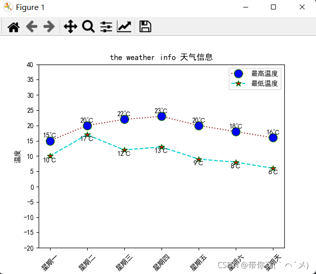
1、折线图
import matplotlib.pyplot as plt
import numpy as np
plt.rcParams["font.sans-serif"] = "SimHei"
plt.rcParams['axes.unicode_minus'] = False
plt.figure()
x = np.arange(1, 8)
y = [15, 20, 22, 23, 20, 18, 16]
y_low = [10, 17, 12, 13, 9, 8, 6]
plt.plot(x, y, color="#A52A2A",
linestyle=':',
marker="o",
markersize=12,
markerfacecolor="b",
markeredgecolor="#006400")
plt.plot(x, y_low,
color="#00CED1",
linestyle='--',
marker="*",
markersize=9,
markerfacecolor="r",
markeredgecolor="#006400"
)
plt.title("the weather info 天气信息")
xtick = ["星期一", "星期二", "星期三", "星期四", "星期五", "星期六", "星期天"]
plt.xticks(x, xtick, rotation=45)
plt.yticks(np.arange(-20, 45, 5))
plt.xlabel("日期")
plt.ylabel("温度")
plt.legend(["最高温度", "最低温度"])
for i, j in zip(x, y):
plt.text(i,
j + 1,
"%d℃" % j,
horizontalalignment='center'
)
for i, j in zip(x, y_low):
plt.text(i,
j - 2,
"%d℃" % j,
horizontalalignment='center'
)
plt.show()
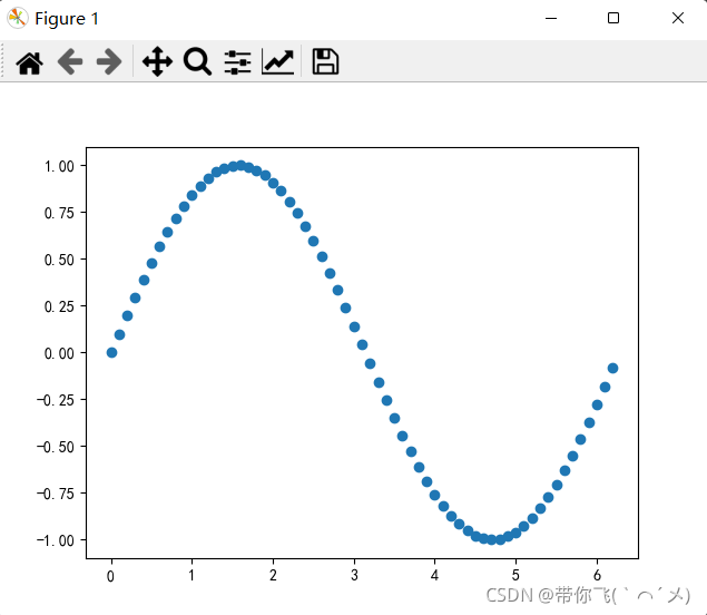
2、散点图
import matplotlib.pyplot as plt
import numpy as np
plt.rcParams["font.sans-serif"] = "SimHei"
plt.rcParams['axes.unicode_minus'] = False
plt.figure()
x = np.arange(0, 2 * np.pi, 0.1)
y = np.sin(x)
plt.scatter(x, y)
plt.show()
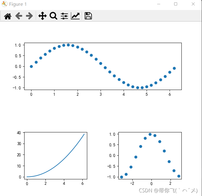
3、子图
import matplotlib.pyplot as plt
import numpy as np
plt.rcParams["font.sans-serif"] = "SimHei"
plt.rcParams['axes.unicode_minus'] = False
fig = plt.figure(figsize=(12, 10), dpi=100)
fig.subplots_adjust(wspace=0.5, hspace=0.9)
x = np.arange(0, 2 * np.pi, 0.2)
fig.add_subplot(2, 1, 1)
y1 = np.sin(x)
plt.scatter(x, y1)
fig.add_subplot(2, 2, 3)
y3 = x ** 2
plt.plot(x, y3)
fig.add_subplot(2, 2, 4)
x4 = np.arange(-np.pi, np.pi, 0.5)
y4 = np.cos(x4)
plt.scatter(x4, y4)
plt.show()