视频学习笔记

Isoforms at the RNA level are readily characterized by cDNA transcript studies.(secondary structures in cellular RNAs)
Alternative RNA splicing
In different human tissues, there are four distinctive isoforms of TH for both TH mRNA and protein. TH mRNA isoforms are produced by differential splicing of a single-copy gene using two splicing donor sites in the first exon and inclusion/exclusion of the second exon. The alternative RNA splicing produces mRNA variants from which proteins are produced that differ in amino acid length, potential phosphorylation, and subtle kinetic properties.
概述
- 预处理
- FASTQC数据质控
- 数据过滤Trimmomatic
- 有参转录组序列比对
- 不同比对软件的比较
- 常用序列比对算法
- 基因组比对
- STAR
- hisat2
- 转录本比对 RSEM
- 无参转录组
- 转录本从头拼接原理
- 拼接方法 Trinity
- 表达定量
- RNA-seq常用统计定量单位
- 基因组比对
- Htseq-Count
- FeatureCount
- 转录本比对 RSEM
- 数据分析
- 思路?
- 差异表达
+ Deseq标准化原理 - 富集分析
+ GO
+ 通路富集分析 - 数据可视化展示
- IGV,基因浏览器
前期准备
- 构建项目目录
	mkdir 00ref 参考序列fasta,注释文件gtf/gff
	mkdir 01raw_data
	mkdir 02clean_data
	mkdir 03align_out
	mkdir 04quantification
	mkdir 05Deqseq ...
- 参考序列/注释信息下载
- Ensembl数据库,JGI数据库,模式植物拟南芥(tair,ARAPORT)
- 原始数据上传,检查完整性md5值
- 给自己的文件生成md5值:
md5sum *gz > md5.txt - 比对已有的md5值(check):
md5sum -c md5.txt
- 给自己的文件生成md5值:
数据预处理
质量控制
- FASTQC
fastqc sample*.gz
for i in `ls *gz` ;do fastqc $i ;done
ls *gz |xargs -I [] echo 'nohup fastqc [] -o ./ &' > fastqc.sh
bash fastqc.sh
multiqc ./
- MultiQC
质量过滤
- Trimmomatic特点:多线程,快。主要用于去除illumina平台接头。根据碱基质量对fastq进行筛选,支持SE/PE,支持gzip/bzip2。
过滤依据:
ILLUMINACLIP:过滤reads中illumina接头
LEADING:reads开头切除质量值低于阈值的碱基
TRAILING:reads末尾切除质量低于阈值碱基
SLIDINGWINDOW:从reads的5‘端滑窗过滤,切除碱基质量平均值低于阈值的滑窗
MINLEN:丢弃剪切后长度低于阈值reads
TOPHRED33:碱基质量体系phred33
TOPHRED64:碱基质量体系phred64
- 接头序列的选择
- “Illumina Single End” / “Illumina Paired End” (看fastqc信息): “TruSeq2-SE.fa” and “TruSeq2-PE.fa”
- “TruSeq Universal Adapter” / “TruSeq Adapter, Index …” (看fastqc信息): “TruSeq3-SE.fa” and “TruSeq3-PE.fa”
- 去接头参数的选择:true(选择),false
trimmomatic PE -threads 4 \
s1_R1.fastq.gz s1_R2.fastq.gz \
cleandata/s1_paired_clean_R1.fastq.gz \
cleandata/s1_unpair_clean_R1.fastq.gz \
cleandata/s1_paired_clean_R2.fastq.gz \
cleandata/s1_unpair_clean_R2.fastq.gz \
ILLUMINACLIP:path/miniconda3/share/trimmomatic-0.36-5/adapters/TruSeq3-PE.fa:2:30:10:1:true \
LEADING:3 TRAILING:3 \
SLIDINGWINDOW:4:20 MINLEN:50 TOPHERD33
序列比对
无参转录组
- 使用拼接工具组装转录本trinity
基于基因组比对(以染色体为单位)
- STAR
- 第一个通过算法优化将比对时间大幅降低的比对工具
- 提供完善的输出内容
- 消耗相对大的内存
- Hisat2
- tophat继任者
- STAR启发下的后起之秀,耗时少内存低
- 缺点:输出结果仅为比对文件,结果单一
基于转录本比对(以转录本为单位)
- RSEM
- 需要提前借助基因组和注释信息准备相关文件
- 结合bowtie2和STAR进行比对和定量分析
STAR实例
- 建立索引
#拟南芥
#build index
STAR --runThreadN 6 --runMode genomeGenerate \#索引模式mode
--genomeDir arab_STAR_genome \
--genomeFastaFiles 00ref/TAIR10.Chr.all.fasta \
--sjdbGTFfile 00ref/Araport11_GFF3_genes_transposons.201606.gtf \
--sjdbOverhang 149#reads长度-1:150-1,用于可变剪切预测?默认100

- 比对
#STAR align 简洁版
STAR --runThreadN 5 --genomeDir arab_STAR_genome \
--readFilesCommand zcat \#文件是gz需要解压缩
--readFilesIn 02clean_data/s1_paired_clean_R1.fastq.gz \
02clean_data/s1_paired_clean_R2.fastq.gz \
--outFileNamePrefix 03align_out/s1_

#STAR align 复杂版
STAR --runThreadN 5 --genomeDir arab_STAR_genome \
--readFilesCommand zcat \#文件是gz需要解压缩
--readFilesIn 02clean_data/s2_paired_clean_R1.fastq.gz \
02clean_data/s2_paired_clean_R2.fastq.gz \
--outFileNamePrefix 03align_out/s2_ \
--outSAMtype BAM SortedByCoordinate \
--outBAMsortingThreadN 5 \
--quantMode TranscriptomeSAM GeneCounts

#--quantMode TranscriptomeSAM will output alignments translated into transcript coordinates, 为了使用RSEM进行定量分析做准备。
–quantMode TranscriptomeSAM
GeneCounts:这个参数需要特别注意,如果你后续要使用RSEM进行定量,就需要添加TranscriptomeSAM,不然生成的BAM文件RSEM无法使用的,GeneCounts生成用于后续featureCounts分析的输入文件
"FATAL ERROR: could not create output file ... Solution: check that you have permission to write this file"
#先查看你的系统打开文件限制数目
$ ulimit -n
1024
#设置一个更大的数目
$ ulimit -n 10000

- 查看比对文件
表达定量
处理原始比对文件
- picard/samtools
- sam转bam
- bam排序
- 去除比对得分较低序列
- 如果需要去除重复reads
三个流程
- STAR+RSEM(先比对再定量)
- 输出结果可以选择转录本定量或基因定量
- 定量单位包括feature count,FPKM,TPM
- 操作相对复杂
- STAR+HTseq(先比对再定量)
- 输出结果为原始read count
- 结果可用于差异表达分析
- 操作相对简单
- Kallisto (free-alignment)
- 速度快省内存
- 基于转录本定量
- 不产生bam不方便后续分析
STAR+RSEM实例
- 准备定量分析所需文件
#rsem prepare reference构建索引文件
rsem-prepare-reference --gtf 00ref/***.gtf \
00ref/***.fasta \
arab_RSEM/arab_rsem

- 利用STAR结果进行定量分析
rsem-calculate-expression --paired-end --no-bam-output \
--alignment -p 5 \
-q 03align_out/s2_Aligned.toTranscriptome.out.bam \
arab_RSEM/arab_rsem \
04rsem_out/s2_rsem

基于基因定量结果,基于转录本定量结果,统计信息目录
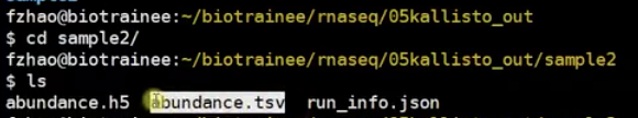
Kallisto实例
- 利用转录本参考序列文件构建索引
kallisto index -I arab_kallisto ../arab_RSEM/arab_rsem.transcripts.fa

- 进行无比对定量分析
kallisto quant -I arab_kallisto/arab_kallisto -o 05kallisto_out/s2 \
02clean_data/s2_paired_clean_R1.fastq.gz \
02clean_data/s2_paired_clean_R2.fastq.gz

Htseq-count
htseq-count -r pos -m union -f bam -s no \
-q 03align_out/s2Aligned.sortedByCoord.out.bam >
05htseq_out/s2.htseq.out
STAR + featureCounts = STAR + HTSeq 升级版
- 安装:
conda install subread优点:速度很快
featureCounts -p -a path/***.gtf -o out.counts.txt -T 6 -t exon -g gene_id *.Aligned.sortedByCoord.out.bam
差异分析
表达定量结果转表达矩阵
- RSEM自带脚本
#构建表达矩阵
rsem-generate-data-matrix *_rsem.genes.results > output.matrix
- 去除所有样本表达量为0的基因
#删除未检测到gene
awk 'BEGIN{printf "geneid\ta1\ta2\tb1\tb2\n"}{if($2+$3+$4+$5>0)print $0}' output.matrix > deseq2_input.txt
edgeR
DESeq2
mkdir 06deseq_out
deseq.r

###查看文件的行数
wc -l output.matrix
wc -l deseq2_input.txt

mv deseq2_input.txt ../06deseq_out/
mv deseq2.r ../06deseq_out/

abundance_estimates_to_matrix.pl
run_DE_analysis.pl
R脚本

### 设置当前目录;
打开一个文件夹中的R脚本,session
或 输入路径;setwd("~/00")


# read.table ,文件有header,第一行为row.name;
input_data <- read.table("deseq2_input.txt", header=TRUE, row.names=1)

# 取整,函数round
input_data <-round(input_data,digits = 0)

# 准备文件
# as.matrix 将输入文件转换为表达矩阵;
input_data <- as.matrix(input_data)

# 控制条件:因子(对照2,实验2)
condition <- factor(c(rep("ct1", 2), rep("exp", 2)))

# input_data根据控制条件构建data.frame
coldata <- data.frame(row.names=colnames(input_data), condition)

library(DESeq2)
# build deseq input matrix 构建输入矩阵
#countData作为矩阵的input_data;colData Data.frame格式;控制条件design;
dds <- DESeqDataSetFromMatrix(countData=input_data,colData=coldata, design=~condition)

# DESeq2 进行差异分析
dds <- DESeq(dds)

#实际包含3步,请自行学习;
# 提取结果
#dds dataset格式转换为DESeq2 中result数据格式,矫正值默认0.1
res <- results(dds,alpha=0.05)
#查看res(DESeqresults格式),可以看到上下调基因
summary(res)

#res(resultset)按照校正后的P值排序
res <- res[order(res$padj), ]
res

# 将进过矫正后的表达量结果加进去;
resdata <- merge(as.data.frame(res), as.data.frame(counts(dds, normalized=TRUE)),by="row.names",sort=FALSE)
names(resdata)[1] <- "Gene"

#查看(resdata)
# output result 输出结果

write.table(resdata,file="diffexpr-results.txt",sep = "\t",quote = F, row.names = F)

#可视化展示
plotMA(res)
maplot <- function (res, thresh=0.05, labelsig=TRUE,...){
with(res,plot(baseMean, log2FoldChange, pch=20, cex=.5, log="x", ...))
with(subset(res, padj<thresh), points(baseMean, log2FoldChange, col="red", pch=20,cex=1.5))

}
png("diffexpr-malot.png",1500,1000,pointsize=20)
maplot(resdata, main="MA Plot")
dev.off()

#画火山图
install.packages("ggrepel")
library(ggplot2)
library(ggrepel)

resdata$significant <- as.factor(resdata$padj<0.05 & abs(resdata$log2FoldChange) > 1)
ggplot(data=resdata, aes(x=log2FoldChange, y =-log10(padj),color =significant)) +
geom_point() +
ylim(0, 8)+
scale_color_manual(values =c("black","red"))+
geom_hline(yintercept = log10(0.05),lty=4,lwd=0.6,alpha=0.8)+
geom_vline(xintercept = c(1,-1),lty=4,lwd=0.6,alpha=0.8)+
theme_bw()+
theme(panel.border = element_blank(),
panel.grid.major = element_blank(),
panel.grid.minor = element_blank(),
axis.line = element_line(colour = "black"))+
labs(title="Volcanoplot_biotrainee (by sunyi)", x="log2 (fold change)",y="-log10 (padj)")+

theme(plot.title = element_text(hjust = 0.5))+
geom_text_repel(data=subset(resdata, -log10(padj) > 6), aes(label=Gene),col="black",alpha =0.8)


差异基因的提取
#查看符合条件的差异基因
awk '{if($3>1 && $7<0.05)print $0}' diffexpr-results.txt |head
#查看差异基因有多少行
awk '{if($3>1 && $7<0.05)print $0}' diffexpr-results.txt |wc -l
#提取某几列
awk '{if($3>1 && $7<0.05)print $0}' diffexpr-results.txt |cut -f 1,2,4,7 |head
#上调基因的提取;
awk '{if($3>1 && $7<0.05)print $0}' diffexpr-results.txt |cut -f 1,2,4,7 > up.gene.txt
#下调基因的提取;
awk '{if($3<-1 && $7<0.05)print $0}' diffexpr-results.txt |cut -f 1,2,4,7 > down.gene.txt

根据第1列是Geneid,第7,8,9,10列是counts数,用awk提取出geneID和counts。
awk -F '\t' '{print $1,$7,$8,$9,$10}' OFS='\t' out_counts.txt >subread_matrix.out