12 _Custom Models and Training with TensorFlow_tensor_ structure_Activation_Layers_huber_Loss_Metric
https://mp.csdn.net/console/editor/html/107294292
Computing Gradients Using Autodiff
To understand how to use autodiff (see https://blog.csdn.net/Linli522362242/article/details/106849041 and https://blog.csdn.net/Linli522362242/article/details/106290394) to compute gradients automatically, let’s consider a simple toy function:
def f(w1, w2):
return 3*w1**2 + 2*w1*w2 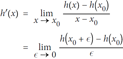
If you know calculus, you can analytically find that the partial derivative of this function with regard to w1 is 6 * w1 + 2 * w2. You can also find that its partial derivative with regard to w2 is 2 * w1. For example, at the point (w1, w2) = (5, 3), these partial derivatives are equal to 36 and 10, respectively, so the gradient vector at this point is (36, 10). But if this were a neural network, the function would be much more complex, typically with tens of thousands of parameters, and finding the partial derivatives analytically by hand would be an almost impossible task. One solution could be to compute an approximation of each partial derivative by measuring how much the function’s output changes when you tweak the corresponding parameter:
w1, w2 = 5,3
eps = 1e-6
( f(w1+eps, w2)-f(w1,w2) )/eps, ( f(w1, w2+eps)-f(w1, w2) )/eps ![]()
Looks about right! This works rather well and is easy to implement, but it is just an approximation, and importantly you need to call f() at least once per parameter (not twice, since we could compute f(w1, w2) just once). Needing to call f() at least once
per parameter makes this approach intractable for large neural networks. So instead, we should use autodiff. TensorFlow makes this pretty simple:
w1, w2 = tf.Variable(5.), tf.Variable(3.)
with tf.GradientTape() as tape:
    z = f(w1,w2)

gradients = tape.gradient(z, [w1,w2])
gradients
We first define two variables w1 and w2, then we create a tf.GradientTape context that will automatically record every operation that involves a variable, and finally we ask this tape to compute the gradients of the result z with regard to both variables [w1, w2]. Let’s take a look at the gradients that TensorFlow computed:
![]()
https://blog.csdn.net/qq_27825451/article/details/89556703
Perfect! Not only is the result accurate (the precision is only limited by the floatingpoint errors), but the gradient() method only goes through the recorded computations once (in reverse order), no matter how many variables there are, so it is
incredibly efficient. It’s like magic!
To save memory, only put the strict minimum inside the tf.GradientTape() block. Alternatively, pause recording by creating a
with tape.stop_recording() block inside the tf.GradientTape() block.
The tape is automatically erased immediately after you call its gradient() method, so you will get an exception if you try to call gradient() twice:
with tf.GradientTape() as tape:
    z=f(w1, w2)

dz_dw1 = tape.gradient(z, w1) # => tensor 36.0
print(dz_dw1)
dz_dw2 = tape.gradient(z, w2) # RuntimeError
print(dz_dw2)
Reason: GradientTape.gradient can only be called once on non-persistent tapes.
If you need to call gradient() more than once, you must make the tape persistent and delete it each time you are done with it to free resources:
with tf.GradientTape(persistent=True) as tape:
    z=f(w1, w2)

dz_dw1 = tape.gradient(z, w1)
print(dz_dw1)
dz_dw2 = tape.gradient(z, w2)## works now!
print(dz_dw2)
del tape![]()
By default, the tape will only track operations involving variables, so if you try to compute the gradient of z with regard to anything other than a variable, the result will be None:
c1, c2 = tf.constant(5.), tf.constant(3.)
with tf.GradientTape() as tape:
    z = f(c1, c2)

gradients = tape.gradient(z,[c1, c2])
gradients![]()
However, you can force the tape to watch any tensors you like, to record every operation that involves them. You can then compute gradients with regard to these tensors, as if they were variables:
c1, c2 = tf.constant(5.), tf.constant(3.)
with tf.GradientTape() as tape:
    tape.watch(c1) ###
    tape.watch(c2) ###
    z = f(c1, c2)

gradients = tape.gradient(z,[c1, c2])
gradients![]()
with tf.GradientTape(persistent=True) as tape:
    z1 = f(w1, w2+2.)
    z2 = f(w1, w2+5.)
    z3 = f(w1, w2+7.)

x=tf.stack([tape.gradient(z, [w1,w2])
                        for z in (z1, z2, z3)
           ])
x 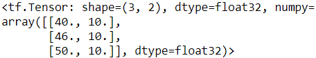
tf.reduce_sum(x, axis=0) ![]()
This can be useful in some cases, like if you want to implement a regularization loss that penalizes activations that vary a lot when the inputs vary little: the loss will be based on the gradient of the activations with regard to the inputs. Since the inputs are not variables, you would need to tell the tape to watch them.
Most of the time a gradient tape is used to compute the gradients of a single value (usually the loss) with regard to a set of values (usually the model parameters). This is where reverse-mode autodiff shines, as it just needs to do one forward pass and one reverse pass to get all the gradients at once. If you try to compute the gradients of a vector, for example a vector containing multiple losses, then TensorFlow will compute the gradients of the vector’s sum. So if you ever need to get the individual gradients (e.g., the gradients of each loss with regard to the model parameters), you must call the tape’s jacobian() method: it will perform reverse-mode autodiff once for each loss in the vector (all in parallel by default). It is even possible to compute second-order partial derivatives (the Hessians, i.e., the partial derivatives of the partial derivatives), but this is rarely needed in practice (see the “Computing Gradients with Autodiff ” section of the notebook for an example).
x, y = tf.Variable(5.), tf.Variable(3.)
def f(x1, x2): # w1, w2 = 5,3
    return 3*x**2 + 2*x*y

with tf.GradientTape( persistent=True ) as hessian_tape:
    with tf.GradientTape() as jacobian_tape:
        z=f(x, y)
    jacobians = jacobian_tape.gradient( z, [x, y] )

hessians = [hessian_tape.gradient(jacobian, [x, y])
            for jacobian in jacobians]

jacobians![]()
hessians[[<tf.Tensor: shape=(), dtype=float32, numpy=6.0>, ###
<tf.Tensor: shape=(), dtype=float32, numpy=2.0>], ###
[<tf.Tensor: shape=(), dtype=float32, numpy=2.0>, None]] ###In some cases you may want to stop gradients from backpropagating through some part of your neural network. To do this, you must use the tf.stop_gradient() function. The function returns its inputs during the forward pass (like tf.identity()), but it does not let gradients through during backpropagation (it acts like a constant):
def f(w1, w2):
    return 3*w1**2 + tf.stop_gradient(2*w1*w2)

with tf.GradientTape() as tape:
    z = f(w1, w2)

tape.gradient(z, [w1, w2])![]()
![]()
tf.math.log(tf.exp( tf.constant(30., dtype=tf.float32))
+1.)![]()
Finally, you may occasionally run into some numerical issues when computing gradients. For example, if you compute the gradients of the my_softplus() function for large inputs, the result will be NaN:
def my_better_softplus(z):
    return tf.where(z>30., z,
                    tf.math.log(tf.exp(z)+1.)
                   )
x = tf.Variable([1000.])
with tf.GradientTape() as tape:
    z = my_better_softplus(x)

z, tape.gradient(z, [x])![]()
This is because computing the gradients of this function using autodiff leads to some numerical difficulties: due to floating-point precision errors, autodiff ends up computing infinity divided by infinity (which returns NaN). Fortunately, we can analytically find that the derivative of the softplus function is just 1 / (1 + 1 / exp(x)), which is numerically stable. Next, we can tell TensorFlow to use this stable function when computing the gradients of the my_softplus() function by decorating it with @tf.custom_gradient and making it return both its normal output and the function that computes the derivatives (note that it will receive as input the gradients that were backpropagated so far, down to the softplus function; and according to the chain rule, we should multiply them with this function’s gradients):
https://www.cnblogs.com/arvin-feng/p/11108799.html
@tf.custom_gradient
def my_better_softplus(z):
    exp = tf.exp(z)

    def my_softplus_gradients(grad):
        return grad / (1+1/exp)

    return tf.math.log(exp+1), my_softplus_gradients
Now when we compute the gradients of the my_better_softplus() function, we get the proper result, even for large input values (however, the main output still explodes because of the exponential; one workaround is to use tf.where() to return the inputs when they are large).
Congratulations! You can now compute the gradients of any function (provided it is differentiable at the point where you compute it), even blocking backpropagation when needed, and write your own gradient functions! This is probably more flexibility than you will ever need, even if you build your own custom training loops, as we will see now.
Custom Training Loops
In some rare cases, the fit() method may not be flexible enough for what you need to do. For example, the Wide & Deep paper we discussed in cp10 https://blog.csdn.net/Linli522362242/article/details/106582512 uses two different optimizers: one for the wide path and the other for the deep path. Since the fit() method only uses one optimizer (the one that we specify when compiling the model), implementing this paper requires writing your own custom loop.
You may also like to write custom training loops simply to feel more confident that they do precisely what you intend them to do (perhaps you are unsure about some details of the fit() method). It can sometimes feel safer to make everything explicit.
However, remember that writing a custom training loop will make your code longer, more error-prone, and harder to maintain.
Unless you really need the extra flexibility, you should prefer using the fit() method rather than implementing your own training loop, especially if you work in a team.
First, let’s build a simple model. No need to compile it, since we will handle the training loop manually:
keras.backend.clear_session()
np.random.seed(42)
tf.random.set_seed(42)

l2_reg = keras.regularizers.l2(0.05)
model = keras.models.Sequential([
    #initilization with he and activation function with Relu and variants
    keras.layers.Dense(30, activation="elu", kernel_initializer="he_normal",
                       kernel_regularizer=l2_reg),
    keras.layers.Dense(1, kernel_regularizer=l2_reg)
])
Next, let’s create a tiny function that will randomly sample a batch of instances from the training set (in Chapter 13 we will discuss the Data API, which offers a much better alternative):
def random_batch(X, y, batch_size=32):
    idx = np.random.randint( len(X), size=batch_size)
    return X[idx], y[idx]
Let’s also define a function that will display the training status, including the number of steps, the total number of steps, the mean loss since the start of the epoch (i.e., we will use the Mean metric to compute it), and other metrics:
def print_status_bar( iteration, total, loss, metrics=None):
    metrics = " - ".join(["{}: {:.4f}".format( m.name, m.result() ) # m is a tensor
                        for m in [loss]
                        + (metrics or [])
                       ])
    end = "" if iteration<total else "\n"
    print("\r{}/{} - ".format(iteration, total) + metrics, end=end)


import time

mean_loss = keras.metrics.Mean(name="loss")
mean_square = keras.metrics.Mean(name="mean_square")

for i in range(1, 50+1):
    loss = 1/i
    mean_loss(loss)
    mean_square(i**2)
    print_status_bar(i, 50, mean_loss, [mean_square])
time.sleep(0.05)![]()
This code is self-explanatory, unless you are unfamiliar with Python string formatting: {:.4f} will format a float with four digits after the decimal point, and using \r (carriage return回车) along with end="" ensures that the status bar always gets printed on the same line. In the notebook, the print_status_bar() function includes a progress bar, but you could use the handy tqdm library instead.
一个叫做“回车”,告诉打字机把打印头定位在左边界,不卷动滚筒;另一个叫做“换行”,告诉打字机把滚筒卷一格,不改变水平位置。
\r (carriage return回车) along with end="\n" 这是回车换行
A fancier[ˈfænsiɚ]华丽点儿的 version with a progress bar:
def progress_bar(iteration, total, size=30):
    running = iteration < total
    c = ">" if running else "="   #size-1 since c used 1
    p = (size - 1) * iteration // total # (6-1)  *3500//10000 ==1
    fmt = "{

   {:{}d}}/{

   {}} [{

   {}}]".format( len(str(total)) ) #{:{}d}#根据len的值预留并补0于前
    #      { :len(str(total))d } /
    params = [iteration, total,
              "="*p + c + "."*(size-p-1)] # format parameter
    return fmt.format(*params)

progress_bar(3500, 10000, size=6)![]()
def print_status_bar( iteration, total, loss, metrics=None):
    metrics = " - ".join(["{}: {:.4f}".format( m.name, m.result() ) # m is a tensor
                        for m in [loss] + (metrics or [])
                       ])
    end = "" if iteration<total else "\n"
    print("\r{} - {}".format(progress_bar(iteration, total),
                             metrics),
          end=end)


mean_loss = keras.metrics.Mean(name="loss")
mean_square = keras.metrics.Mean(name="mean_square")

for i in range(1, 50+1):
    loss = 1/i
    mean_loss(loss)
    mean_square(i**2)
    print_status_bar(i, 50, mean_loss, [mean_square])
time.sleep(0.05)![]()
With that, let’s get down to business! First, we need to define some hyperparameters and choose the optimizer, the loss function, and the metrics (just the MAE in this example):
keras.backend.clear_session()
np.random.seed(42)
tf.random.set_seed(42)

n_epochs = 5
batch_size = 32
n_steps = len(X_train) // batch_size # 11610//32 =362

#https://blog.csdn.net/Linli522362242/article/details/107086444
optimizer = keras.optimizers.Nadam(lr=0.01)
loss_fn = keras.losses.mean_squared_error
mean_loss = keras.metrics.Mean()
metrics = [keras.metrics.MeanAbsoluteError()]
And now we are ready to build the custom loop!
def progress_bar(iteration, total, size=30):
    running = iteration < total
    c = ">" if running else "="
    p = (size - 1) * iteration // total # (6-1)*3500 //10000 ==1
    fmt = "{

   {:{}d}}/{

   {}} [{

   {}}]".format( len(str(total)) )
    #      { :len(str(total))d } /
    params = [iteration, total,
              "="*p + c + "."*(size-p-1)]
    return fmt.format(*params)

def print_status_bar( iteration, total, loss, metrics=None):
    metrics = " - ".join(["{}: {:.4f}".format( m.name, m.result() ) # m is a tensor
                        for m in [loss]
                        + (metrics or [])
                       ])
    end = "" if iteration<total else "\n"
    print("\r{} - {}".format(progress_bar(iteration, total),
                             metrics),
          end=end)
keras.backend.clear_session()
np.random.seed(42)
tf.random.set_seed(42)
n_epochs = 5
batch_size = 32
n_steps = len(X_train) // batch_size # 11610//32 =362
#https://blog.csdn.net/Linli522362242/article/details/107086444
# optimizer, loss, metrics
optimizer = keras.optimizers.Nadam(lr=0.01)
loss_fn = keras.losses.mean_squared_error # ==import keras.losses.mean_squared_error as loss_fn
mean_loss = keras.metrics.Mean()
metrics = [keras.metrics.MeanAbsoluteError()] ### [ ]
def random_batch(X, y, batch_size=32):
idx = np.random.randint( len(X), size=batch_size)
return X[idx], y[idx]
model = keras.models.Sequential([
#initilization with he and activation function with Relu and variants
keras.layers.Dense(30, activation="elu", kernel_initializer="he_normal",
kernel_regularizer=l2_reg),
keras.layers.Dense(1, kernel_regularizer=l2_reg)
])
for epoch in range(1, n_epochs+1):
print( "Epoch {}/{}".format(epoch, n_epochs) )
for step in range(1, n_steps+1): # n_steps = len(X_train) // batch_size
X_batch, y_batch = random_batch(X_train_scaled, y_train)
with tf.GradientTape() as tape:
# make a prediction for one batch (using the model as a function)
y_pred = model(X_batch) #input X_batch to the model
# loss_fn = keras.losses.mean_squared_error
main_loss = tf.reduce_mean( loss_fn(y_batch, y_pred) )#returns one loss per batch
# https://www.tensorflow.org/api_docs/python/tf/math/add_n
# model.losses: there is one "regularization loss" per layer).
# The regularization losses are already reduced to a single scalar each
loss = tf.add_n([main_loss]+model.losses)
# compute the gradient of the loss with regard to each trainable variable
gradients = tape.gradient(loss, model.trainable_variables)
optimizer.apply_gradients( zip(gradients, model.trainable_variables) ) # to minimize
######################## constraint ########################
# If you add weight constraints to your model (e.g., by setting kernel_constraint
# or bias_constraint when creating a layer), you should update the training loop to
# apply these constraints just after apply_gradients():
        for variable in model.variables:
            if variable.constraint is not None:
                variable.assign( variable.constraint(variable) )
# Then we update the mean loss and the metrics (over the current epoch)
mean_loss(loss) # keras.metrics.Mean()
for metric in metrics:
metric(y_batch, y_pred) # metrics = [keras.metrics.MeanAbsoluteError()]
# we display the status bar
print_status_bar( step*batch_size, len(y_train), mean_loss, metrics)
# At the end of each epoch, we display the status bar again to make it look complete
# and to print a line feed, and we reset the states of the mean loss and the metrics.
print_status_bar( len(y_train), len(y_train), mean_loss, metrics)
for metric in [mean_loss] + metrics:
metric.reset_states()
There’s a lot going on in this code, so let’s walk through it:
- We create two nested loops: one for the epochs, the other for the batches within an epoch.
- Then we sample a random batch from the training set.
- Inside the tf.GradientTape() block, we make a prediction for one batch (using the model as a function), and we compute the loss: it is equal to the main loss plus the other losses (in this model, there is one regularization loss per layer). Since the mean_squared_error() function returns one loss per instance, we compute the mean over the batch using tf.reduce_mean() (if you wanted to apply different weights to each instance, this is where you would do it). The regularization losses are already reduced to a single scalar each, so we just need to sum them (using tf.add_n(), which sums multiple tensors of the same shape and data type).
- Next, we ask the tape to compute the gradient of the loss with regard to each trainable variable (not all variables!), and we apply them to the optimizer to perform a Gradient Descent step.
- Then we update the mean loss and the metrics (over the current epoch), and we display the status bar.
- At the end of each epoch, we display the status bar again to make it look complete and to print a line feed, and we reset the states of the mean loss and the metrics.
If you set the optimizer’s clipnorm or clipvalue hyperparameter
https://blog.csdn.net/Linli522362242/article/details/106935910, it will take care of this for you. If you want to apply any other transformation to the gradients, simply do so before calling the apply_gradients() method.
If you add weight constraints to your model (e.g., by setting kernel_constraint or bias_constraint when creating a layer), you should update the training loop to apply these constraints just after apply_gradients():
for variable in model.variables:
if variable.constraint is not None:
variable.assign( variable.constraint(variable) )Most importantly, this training loop does not handle layers that behave differently during training and testing (e.g., BatchNormalization or Dropout). To handle these, you need to call the model with training=True and make sure it propagates this to every layer that needs it.
As you can see, there are quite a lot of things you need to get right, and it’s easy to make a mistake. But on the bright side, you get full control, so it’s your call.
try:
    from tqdm.notebook import trange
    from collections import OrderedDict
    with trange(1, n_epochs + 1, desc="All epochs") as epochs:
        for epoch in epochs:
            with trange(1, n_steps + 1, desc="Epoch {}/{}".format(epoch, n_epochs)) as steps:
                for step in steps:
                    X_batch, y_batch = random_batch(X_train_scaled, y_train)
                    with tf.GradientTape() as tape:
                        y_pred = model(X_batch)
                        main_loss = tf.reduce_mean(loss_fn(y_batch, y_pred))
                        loss = tf.add_n([main_loss] + model.losses)
                    gradients = tape.gradient(loss, model.trainable_variables)
                    optimizer.apply_gradients(zip(gradients, model.trainable_variables))
                    for variable in model.variables:
                        if variable.constraint is not None:
                            variable.assign(variable.constraint(variable))
                    status = OrderedDict()
                    mean_loss(loss)
                    status["loss"] = mean_loss.result().numpy()
                    for metric in metrics:
                        metric(y_batch, y_pred)
                        status[metric.name] = metric.result().numpy()
                    steps.set_postfix(status)
            for metric in [mean_loss] + metrics:
                metric.reset_states()
except ImportError as ex:
    print("To run this cell, please install tqdm, ipywidgets and restart Jupyter")
Now that you know how to customize any part of your models and training algorithms, let’s see how you can use TensorFlow’s automatic graph generation feature: it can speed up your custom code considerably, and it will also make it portable to any platform supported by TensorFlow (see Chapter 19).
TensorFlow Functions and Graphs
In TensorFlow 1, graphs were unavoidable (as were the complexities that came with them) because they were a central part of TensorFlow’s API. In TensorFlow 2, they are still there, but not as central, and they’re much (much!) simpler to use. To show just how simple, let’s start with a trivial function that computes the cube of its input:
def cube(x):
    return x**3
We can obviously call this function with a Python value, such as an int or a float, or we can call it with a tensor:
cube(2)![]()
cube( tf.constant(2.0) )![]()
Now, let’s use tf.function() to convert this Python function to a TensorFlow Function:
tf_cube = tf.function(cube)
tf_cube![]()
This TF Function can then be used exactly like the original Python function, and it will return the same result (but as tensors):
tf_cube(2)![]()
tf_cube( tf.constant(2.0))![]()
tf_cube( tf.constant(2))![]()
Under the hood, tf.function() analyzed the computations performed by the cube() function and generated an equivalent computation graph! As you can see, it was rather painless (we will see how this works shortly). Alternatively, we could have used tf.function as a decorator; this is actually more common:
@tf.function
def tf_cube(x):
    return x**3

tf_cube(2.0)![]()
![]()
![]()
![]()
tf_cube.python_function(2.0)![]()
tf_cube(0.5)![]()
![]()
![]()
![]()
TensorFlow optimizes the computation graph, pruning unused nodes, simplifying expressions (e.g., 1 + 2 would get replaced with 3), and more. Once the optimized graph is ready, the TF Function efficiently executes the operations in the graph, in the appropriate order (and in parallel when it can). As a result, a TF Function will usually run much faster than the original Python function, especially if it performs complex computations. Most of the time you will not really need to know more than that: when you want to boost a Python function, just transform it into a TF Function. That’s all!
Moreover, when you write a custom loss function, a custom metric, a custom layer, or any other custom function and you use it in a Keras model (as we did throughout this chapter), Keras automatically converts your function into a TF Function—no need to use tf.function(). So most of the time, all this magic is 100% transparent.
You can tell Keras not to convert your Python functions to TF Functions by setting dynamic=True when creating a custom layer or a custom model. Alternatively, you can set run_eagerly=True when calling the model’s compile() method.
tf_cube(tf.constant([10,20]))![]()
tf_cube(tf.constant([10,20])).shape ![]()
By default, a TF Function generates a new graph for every unique set of input shapes and data types and caches it for subsequent calls. For example, if you call tf_cube(tf.constant(10)), a graph will be generated for int32 tensors of shape [].
Then if you call tf_cube(tf.constant(20)), the same graph will be reused. But if you then call tf_cube(tf.constant([10, 20])), a new graph will be generated for int32 tensors of shape [2]. This is how TF Functions handle polymorphism (i.e., varying argument types and shapes). However, this is only true for tensor arguments: if you pass numerical Python values to a TF Function, a new graph will be generated for every distinct value: for example, calling tf_cube(10) and tf_cube(20) will generate two graphs.
If you call a TF Function many times with different numerical Python values, then many graphs will be generated, slowing down your program and using up a lot of RAM (you must delete the TF Function to release it). Python values should be reserved for arguments that will have few unique values, such as hyperparameters like the number of neurons per layer. This allows TensorFlow to better optimize each variant of your model.
AutoGraph and Tracing
So how does TensorFlow generate graphs? It starts by analyzing the Python function’s source code to capture all the control flow statements, such as for loops, while loops, and if statements, as well as break, continue, and return statements. This first step is called AutoGraph. The reason TensorFlow has to analyze the source code is that Python does not provide any other way to capture control flow statements: it offers magic methods like __add__() and __mul__() to capture operators like + and *, but there are no __while__() or __if__() magic methods. After analyzing the function’s code, AutoGraph outputs an upgraded version of that function in which all the control flow statements are replaced by the appropriate TensorFlow operations, such as
tf.while_loop() for loops and tf.cond() for if statements. For example, in Figure 12-4, AutoGraph analyzes the source code of the sum_squares() Python function, and it generates the tf__sum_squares() function. In this function, the for loop is replaced by the definition of the loop_body() function (containing the body of the original for loop), followed by a call to the for_stmt() function. This call will build the appropriate tf.while_loop() operation in the computation graph.
Figure 12-4. How TensorFlow generates graphs using AutoGraph and tracing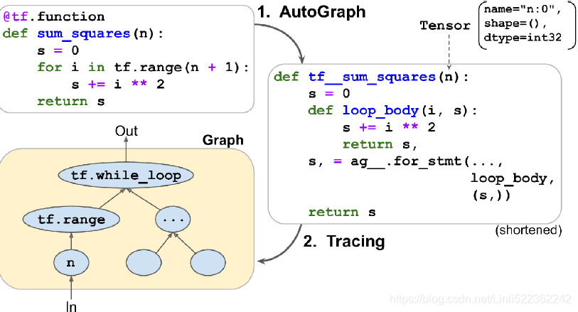
Next, TensorFlow calls this “upgraded” function, but instead of passing the argument, it passes a symbolic tensor符号张量—a tensor without any actual value, only a name, a data type, and a shape. For example, if you call sum_squares(tf.constant(10)), then the tf__sum_squares() function will be called with a symbolic tensor of type int32 and shape []. The function will run in graph mode, meaning that each TensorFlow operation will add a node in the graph to represent itself and its output tensor(s) (as opposed to the regular mode, called eager execution, or eager mode). In graph mode, TF operations do not perform any computations. This should feel familiar if you know TensorFlow 1, as graph mode was the default mode. In Figure 12-4, you can see the tf__sum_squares() function being called with a symbolic tensor as its argument (in this case, an int32 tensor of shape []) and the final graph being generated during tracing. The nodes represent operations, and the arrows represent tensors (both the generated function and the graph are simplified).
To view the generated function’s source code, you can call tf.auto graph.to_code(sum_squares.python_function). The code is not meant to be pretty, but it can sometimes help for debugging.
TF Function Rules
Most of the time, converting a Python function that performs TensorFlow operations into a TF Function is trivial: decorate it with @tf.function or let Keras take care of it for you. However, there are a few rules to respect:
- If you call any external library, including NumPy or even the standard library, this call will run only during tracing; it will not be part of the graph. Indeed, a TensorFlow graph can only include TensorFlow constructs (tensors, operations, variables, datasets, and so on). So, make sure you use tf.reduce_sum() instead of np.sum(), tf.sort() instead of the built-in sorted() function, and so on (unless you really want the code to run only during tracing). This has a few additional implications:
—If you define a TF Function f(x) that just returns np.random.rand(), a random number will only be generated when the function is traced, so f(tf.constant(2.)) and f(tf.constant(3.)) will return the same random number, but f(tf.constant([2., 3.])) will return a different one. If you replace np.random.rand() with tf.random.uniform([]), then a new random number
will be generated upon every call, since the operation will be part of the graph.@tf.function def f(x): return np.random.rand()
Reason: a TensorFlow graph can only include TensorFlow constructs (tensors, operations, variables, datasets, and so on)
VS
Reason: NumPy or even the standard library, this call will run only during tracing; it will not be part of the graph
f(tf.constant([2.,3.]))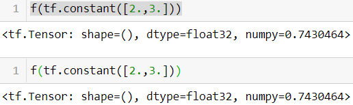
@tf.function
def f(x):
    return tf.random.uniform([])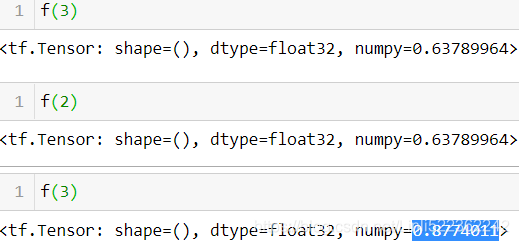
VS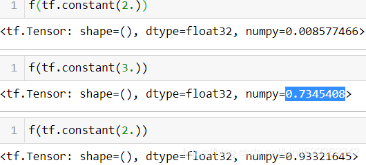

Reason: If you replace np.random.rand() with tf.random.uniform([]), then a new random number
will be generated upon every call, since the operation will be part of the graph.
—If your non-TensorFlow code has side effects (such as logging something or updating a Python counter), then you should not expect those side effects to occur every time you call the TF Function, as they will only occur when the function is traced.
—You can wrap arbitrary Python code in a tf.py_function() operation, but doing so will hinder performance, as TensorFlow will not be able to do any graph optimization on this code. It will also reduce portability, as the graph will only run on platforms where Python is available (and where the right libraries are installed).
- You can call other Python functions or TF Functions, but they should follow the same rules, as TensorFlow will capture their operations in the computation graph. Note that these other functions do not need to be decorated with @tf.function.
- If the function creates a TensorFlow variable (or any other stateful TensorFlow object https://blog.csdn.net/Linli522362242/article/details/107294292, such as a dataset or a queue), it must do so upon the very first call, and only then, or else you will get an exception. It is usually preferable to create variables outside of the TF Function (e.g., in the build() method of a custom layer). If you want to assign a new value to the variable, make sure you call its assign() method, instead of using the = operator.
- The source code of your Python function should be available to TensorFlow. If the source code is unavailable (for example, if you define your function in the Python shell, which does not give access to the source code, or if you deploy only the compiled *.pyc Python files to production), then the graph generation process will fail or have limited functionality.
- TensorFlow will only capture for loops that iterate over a tensor or a dataset. So make sure you use for i in tf.range(x) rather than for i in range(x), or else the loop will not be captured in the graph. Instead, it will run during tracing. (This may be what you want if the for loop is meant to build the graph, for example to create each layer in a neural network.)
It’s time to sum up! In this chapter we started with a brief overview of TensorFlow, then we looked at TensorFlow’s low-level API, including tensors, operations, variables, and special data structures. We then used these tools to customize almost every
component in tf.keras. Finally, we looked at how TF Functions can boost performance, how graphs are generated using AutoGraph and tracing, and what rules to follow when you write TF Functions (if you would like to open the black box a bit
further, for example to explore the generated graphs, you will find technical details in Appendix G).
TF Functions and Concrete具体 Functions
TF Functions are polymorphic多态的, meaning they support inputs of different types (and shapes). For example, consider the following tf_cube() function:
@tf.function
def tf_cube(x):
    return x**3
Every time you call a TF Function with a new combination of input types or shapes, it generates a new concrete function, with its own graph specialized for this particular combination. Such a combination of argument types and shapes is called an input signature. If you call the TF Function with an input signature it has already seen before, it will reuse the concrete function it generated earlier. For example, if you call tf_cube(tf.constant(3.0)), the TF Function will reuse the same concrete function it used for tf_cube(tf.constant(2.0)) (for float32 scalar tensors).
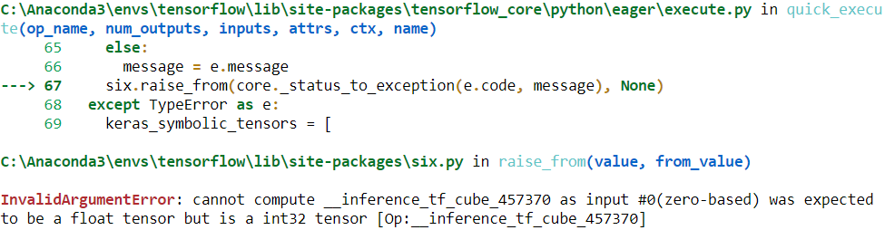
tf_cube(2) ![]()
tf_cube(tf.constant(2)) ![]()
tf_cube(tf.constant(2.0))![]()
tf_cube(tf.constant(3.0))![]()
But it will generate a new concrete function if you call tf_cube(tf.constant([2.0])) or tf_cube(tf.constant([3.0])) (for float32 tensors of shape [1]),
tf_cube(tf.constant([2.0]))![]()
tf_cube(tf.constant([3.0]))![]()
and yet another for tf_cube(tf.constant([[1.0, 2.0], [3.0, 4.0]])) (for float32 tensors of shape [2, 2]). You can get the concrete function for a particular combination of inputs by calling the TF Function’s get_concrete_function() method. It can then be called like a regular function, but it will only support one input signature (in this example, float32 scalar tensors):
concrete_function = tf_cube.get_concrete_function(tf.constant(2.0)
                                                 )
concrete_function.graph![]()
concrete_function(tf.constant(2.0)) ![]()
concrete_function(tf.constant(2))
... ...
but it will only support one input signature (in this example, float32 scalar tensors):
concrete_function is tf_cube.get_concrete_function(tf.constant(2.0)) ![]()
Figure G-1 shows the tf_cube() TF Function, after we called tf_cube(2) and tf_cube(tf.constant(2.0)): two concrete functions were generated, one for each signature, each with its own optimized function graph (FuncGraph), and its own function
definition (FunctionDef). A function definition points to the parts of the graph that correspond to the function’s inputs and outputs. In each FuncGraph, the nodes (ovals) represent operations (e.g., power, constants, or placeholders for arguments
like x), while the edges (the solid arrows between the operations) represent the tensors that will flow through the graph. The concrete function on the left is specialized for x = 2, so TensorFlow managed to simplify it to just output 8 all the time (note that the function definition does not even have an input). The concrete function on the right is specialized for float32 scalar tensors, and it could not be simplified. If we call tf_cube(tf.constant(5.0)), the second concrete function will be called, the placeholder operation for x will output 5.0, then the power operation will compute 5.0 ** 3, so the output will be 125.0.
Figure G-1. The tf_cube() TF Function, with its ConcreteFunctions and their Function‐Graphs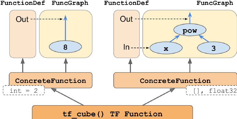
The tensors in these graphs are symbolic tensors, meaning they don’t have an actual value, just a data type, a shape, and a name. They represent the future tensors that will flow through the graph once an actual value is fed to the placeholder x and the graph is executed. Symbolic tensors make it possible to specify ahead of time how to connect operations, and they also allow TensorFlow to recursively infer the data types and shapes of all tensors, given the data types and shapes of their inputs.
Now let’s continue to peek under the hood, and see how to access function definitions and function graphs and how to explore a graph’s operations and tensors.
Exploring Function Definitions and Graphs
You can access a concrete function’s computation graph using the graph attribute, and get the list of its operations by calling the graph’s get_operations() method:
concrete_function.graph ![]()
ops = concrete_function.graph.get_operations()
ops 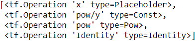
In this example, the first operation represents the input argument x (it is called a placeholder), the second “operation” represents the constant 3### x**3 ###, the third operation represents the power operation (**), and the final operation represents the output of this function (it is an identity operation, meaning it will do nothing more than copy the output of the addition operation). Each operation has a list of input and output tensors that you can easily access using the operation’s inputs and outputs attributes.
For example, let’s get the list of inputs and outputs of the power operation:
pow_op = ops[2]
list(pow_op.inputs)# OR pow_op.inputs ![]()
pow_op.inputs ![]()
pow_op.outputs ![]()
This computation graph is represented in Figure G-2.
Figure G-2. Example of a computation graph

The tensors in these graphs are symbolic tensors, meaning they don’t have an actual value, just a data type, a shape, and a name.
Note that each operation has a name. It defaults to the name of the operation (e.g., "pow"), but you can define it manually when calling the operation (e.g., tf.pow(x, 3, name="other_name")). If a name already exists, TensorFlow automatically adds a
unique index (e.g., "pow_1", "pow_2", etc.). Each tensor also has a unique name: it is always the name of the operation that outputs this tensor, plus :0 if it is the operation’s first output, or :1 if it is the second output, and so on. You can fetch an operation or a tensor by name using the graph’s get_operation_by_name() or get_tensor_by_name() methods:
concrete_function.graph.get_operation_by_name('x') ![]()
concrete_function.graph.get_tensor_by_name('Identity:0') ![]()
concrete_function.graph.get_operation_by_name('Identity:0')
The concrete function also contains the function definition (represented as a protocol buffer), which includes the function’s signature. This signature allows the concrete function to know which placeholders to feed with the input values, and which tensors to return:
concrete_function.function_def.signature 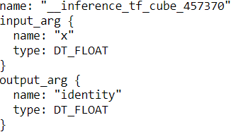
Now let’s look more closely at tracing.
A Closer Look at Tracing
Let’s tweak the tf_cube() function to print its input
@tf.function
def tf_cube(x):
    print("x=", x)
    return x**3
Now let’s call it:
result = tf_cube( tf.constant(2.0) ) ![]()
result ![]()
The result looks good, but look at what was printed: x is a symbolic tensor! It has a shape and a data type, but no value. Plus it has a name ("x:0"). This is because the print() function is not a TensorFlow operation, so it will only run when the Python function is traced, which happens in graph mode, with arguments replaced with symbolic tensors (same type and shape, but no value). Since the print() function was not captured into the graph, the next times we call tf_cube() with float32 scalar tensors, nothing is printed:
result = tf_cube(2) # new Python value: trace!
result = tf_cube(3) # new Python value: trace!
result = tf_cube( tf.constant([[1., 2.]
                              ])
                ) # New shape: trace!
result = tf_cube( tf.constant([[3., 4.],
                               [5., 6.]
                              ])
                ) # new shape: trace!
result = tf_cube( tf.constant([[7., 8.],
                               [9., 10.],
                               [11., 12.]
                              ])
                ) # new shape: trace!
result = tf_cube( tf.constant([[7., 8.],
                               [9., 19.]
                              ])
                )# Same shape: no trace
No print action!
If your function has Python side effects (e.g., it saves some logs to disk), be aware that this code will only run when the function is traced (i.e., every time the TF Function is called with a new input signature). It best to assume that the function may be traced (or not) any time the TF Function is called.
In some cases, you may want to restrict a TF Function to a specific input signature. For example, suppose you know that you will only ever call a TF Function with batches of 28 × 28–pixel images, but the batches will have very different sizes. You
may not want TensorFlow to generate a different concrete function for each batch size, or count on it to figure out on its own when to use None. In this case, you can specify the input signature like this:
@tf.function(input_signature=[ tf.TensorSpec([None, 28, 28], tf.float32) ])
def shrink(images):
    print("Tracing", images)
    return images[:, ::2, ::2] # drop half the rows and columns
This TF Function will accept any float32 tensor of shape [*, 28, 28], and it will reuse the same concrete function every time:
img_batch_1 = tf.random.uniform(shape=[100, 28, 28])
img_batch_2 = tf.random.uniform(shape=[50, 28, 28])
preprocessed_images = shrink(img_batch_1) # Works fine. Traces the function
preprocessed_images = shrink(img_batch_2) # Reuses the same concrete function########## ![]()
However, if you try to call this TF Function with a Python value, or a tensor of an unexpected data type or shape, you will get an exception:
img_batch_3 = tf.random.uniform(shape=[2,2,2])
preprocessed_images = shrink(img_batch_3) # rejects unexpected types or shapes
... ...
img_batch_3 = tf.random.uniform(shape=[2,2,2])
try:
    preprocessed_images = shrink(img_batch_3) # rejects unexpected types or shapes
except ValueError as ex:
    print(ex)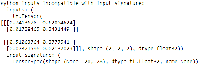
Using AutoGraph to Capture Control Flow
If your function contains a simple for loop, what do you expect will happen? For example, let’s write a function that will add 10 to its input, by just adding 1 10 times:
A "static" for loop using range():
@tf.function
def add_10(x):
    for i in range(10):
        x += 1
    return x

add_10(tf.constant(5)) ![]()
It works fine, but when we look at its graph, we find that it does not contain a loop: it just contains 10 addition operations!
add_10.get_concrete_function(tf.constant(5)).graph.get_operations() This actually makes sense: when the function got traced, the loop ran 10 times, so the x += 1 operation was run 10 times, and since it was in graph mode, it recorded this operation 10 times in the graph. You can think of this for loop as a “static” loop that gets unrolled when the graph is created.
If you want the graph to contain a “dynamic” loop instead (i.e., one that runs when the graph is executed), you can create one manually using the tf.while_loop() operation, but it is not very intuitive (see the “Using AutoGraph to Capture Control Flow”
section of the Chapter 12 notebook for an example). Instead, it is much simpler to use TensorFlow’s AutoGraph feature, discussed in Chapter 12. AutoGraph is actually activated by default (if you ever need to turn it off, you can pass autograph=False to tf.function()). So if it is on, why didn’t it capture the for loop in the add_10() function? Well, it only captures for loops that iterate over tf.range(), not range(). This is to give you the choice:
- If you use range(), the for loop will be static, meaning it will only be executed when the function is traced. The loop will be “unrolled” into a set of operations for each iteration, as we saw.
- If you use tf.range(), the loop will be dynamic, meaning that it will be included in the graph itself (but it will not run during tracing).
A "dynamic" loop using tf.while_loop():
如果用伪代码来表示运行逻辑的话,那 tf.while_loop 的功能与下面的代码相当 :
def while_loop(cond, loop_body, init_state):
    state = init_state     # 为循环的起始状态
    while(cond(state)) :   # 使用cond函数判断是否达到循环结束条件。
        state = loop_body(state)   # 使用loop_body函数对state进行更新。
    return state
A "dynamic" loop using tf.while_loop():
@tf.function
def add_10(x):
    condiction = lambda i, x: tf.less(i, 10) # i<10
    body = lambda i, x: ( tf.add(i,1), tf.add(x,1) ) #i+1, x+1
                                                         #init_state
    final_i, final_x = tf.while_loop( condiction, body, [tf.constant(0), x])
    return final_x

add_10( tf.constant(5) )![]()
add_10.get_concrete_function(tf.constant(5)).graph.get_operations()[<tf.Operation 'x' type=Placeholder>,
<tf.Operation 'Const' type=Const>, # +1
<tf.Operation 'while/maximum_iterations' type=Const>, # 10
<tf.Operation 'while/loop_counter' type=Const>, # i
<tf.Operation 'while' type=StatelessWhile>, # i, x
<tf.Operation 'Identity' type=Identity>]As you can see, the graph now contains a While loop operation, as if you had called the tf.while_loop() function.
A "dynamic" for loop using tf.range() (captured by autograph):
@tf.function
def add_10(x):
    for i in tf.range(10):
        x = x+1
    return x

add_10.get_concrete_function(tf.constant(0)).graph.get_operations()
[<tf.Operation 'x' type=Placeholder>,
<tf.Operation 'range/start' type=Const>, # 0
<tf.Operation 'range/limit' type=Const>, # 10
<tf.Operation 'range/delta' type=Const>, # +1
<tf.Operation 'range' type=Range>,
<tf.Operation 'while/maximum_iterations' type=Const>, #10
<tf.Operation 'while/loop_counter' type=Const>, # i
<tf.Operation 'while' type=StatelessWhile>, #i,x
<tf.Operation 'Identity' type=Identity>]Handling Variables and Other Resources in TF Functions
In TensorFlow, variables and other stateful objects, such as queues or datasets, are called resources. TF Functions treat them with special care: any operation that reads or updates a resource is considered stateful, and TF Functions ensure that stateful operations are executed in the order they appear (as opposed to stateless operations, which may be run in parallel, so their order of execution is not guaranteed). Moreover, when you pass a resource as an argument to a TF Function, it gets passed by reference, so the function may modify it.
For example:
counter = tf.Variable(0)

@tf.function
def increment(counter, c=1):
    return counter.assign_add(c) #############

increment(counter) # counter is now equal to 1
increment(counter) # counter is now equal to 2 ![]()
If you peek at the function definition, the first argument is marked as a resource:
function_def = increment.get_concrete_function(counter).function_def
function_def
signature {
name: "__inference_increment_164"
input_arg {
name: "counter"
type: DT_RESOURCE
}
output_arg {
name: "identity"
type: DT_INT32
}
is_stateful: true
control_output: "AssignAddVariableOp"
control_output: "ReadVariableOp"
}
node_def {
name: "Const"
op: "Const"
attr {
key: "dtype"
value {
type: DT_INT32
}
}
attr {
key: "value"
value {
tensor {
dtype: DT_INT32
tensor_shape {
}
int_val: 1
}
}
}
experimental_debug_info {
original_node_names: "Const"
}
}
node_def {
name: "AssignAddVariableOp"
op: "AssignAddVariableOp"
input: "counter"
input: "Const:output:0"
attr {
key: "dtype"
value {
type: DT_INT32
}
}
experimental_debug_info {
original_node_names: "AssignAddVariableOp"
}
}
node_def {
name: "ReadVariableOp"
op: "ReadVariableOp"
input: "counter"
input: "^AssignAddVariableOp"
attr {
key: "dtype"
value {
type: DT_INT32
}
}
experimental_debug_info {
original_node_names: "ReadVariableOp"
}
}
node_def {
name: "Identity"
op: "Identity"
input: "ReadVariableOp:value:0"
input: "^AssignAddVariableOp"
input: "^ReadVariableOp"
attr {
key: "T"
value {
type: DT_INT32
}
}
experimental_debug_info {
original_node_names: "Identity"
}
}
ret {
key: "identity"
value: "Identity:output:0"
}
control_ret {
key: "AssignAddVariableOp"
value: "AssignAddVariableOp"
}
control_ret {
key: "ReadVariableOp"
value: "ReadVariableOp"
}
arg_attr {
value {
attr {
key: "_user_specified_name"
value {
s: "counter"
}
}
}
}
function_def = increment.get_concrete_function(counter).function_def
function_def.signature.input_arg[0] ![]()
It is also possible to use a tf.Variable defined outside of the function, without explicitly passing it as an argument:
counter = tf.Variable(0)

@tf.function
def increment(c=1):
    return counter.assign_add(c)

increment()
increment() ![]()
function_def = increment.get_concrete_function().function_def
function_def.signature.input_arg[0] ![]()
The TF Function will treat this as an implicit first argument, so it will actually end up with the same signature (except for the name of the argument). However, using global variables can quickly become messy, so you should generally wrap variables (and other resources) inside classes. The good news is @tf.function works fine with methods too:
class Counter:
    def __init__(self):
        self.counter = tf.Variable(0)###

    @tf.function
    def increment(self, c=1):
        return self.counter.assign_add(c)###

c = Counter()
c.increment()
c.increment() ![]()
Do not use =, +=, -=, or any other Python assignment operator with TF variables. Instead, you must use the assign(), assign_add(), or assign_sub() methods. If you try to use a Python assignment operator, you will get an exception when you call the method.
@tf.function
def add_10(x):
    for i in tf.range(10):
        x += 1
    return x

# To view the generated function’s source code
tf.autograph.to_code( add_10.python_function )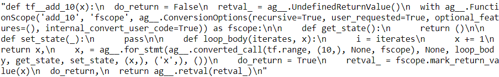
def display_tf_code(func):
    from IPython.display import display, Markdown

    if hasattr(func, "python_function"):
        func = func.python_function

    code = tf.autograph.to_code(func)
    display(Markdown('```python\n{}\n```'.format(code)))

display_tf_code(add_10) 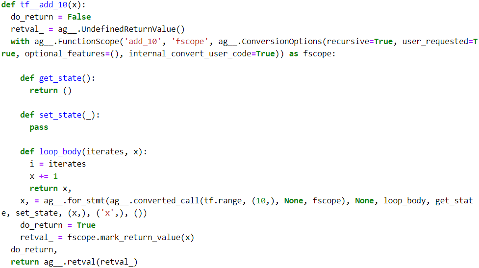
A good example of this object-oriented approach is, of course, tf.keras. Let’s see how to use TF Functions with tf.keras.
https://blog.csdn.net/Linli522362242/article/details/107596098
In the next chapter, we will look at how to efficiently load and preprocess data with TensorFlow.
Exercises
1. How would you describe TensorFlow in a short sentence? What are its main features? Can you name other popular Deep Learning libraries?
TensorFlow is an open-source library for numerical computation, particularly well suited and fine-tuned for large-scale Machine Learning. Its core is similar to NumPy, but it also features GPU support, support for distributed computing, computation graph analysis and optimization capabilities (with a portable graph format that allows you to train a TensorFlow model in one environment and run it in another), an optimization API based on reverse-mode autodiff, and several powerful APIs such as tf.keras, tf.data, tf.image, tf.signal, and more. Other popular Deep Learning libraries include PyTorch, MXNet, Microsoft Cognitive Toolkit, Theano, Caffe2, and Chainer.
2. Is TensorFlow a drop-in replacement for NumPy? What are the main differences between the two?
Although TensorFlow offers most of the functionalities provided by NumPy, it is not a drop-in replacement, for a few reasons. First, the names of the functions are not always the same (for example, tf.reduce_sum() versus np.sum()). Second, some functions do not behave in exactly the same way (for example, tf.transpose() creates a transposed copy of a tensor, while NumPy’s T attribute creates a transposed view, without actually copying any data). Lastly, NumPy arrays are mutable, while TensorFlow tensors are not (but you can use a tf.Variable if you need a mutable object).
3. Do you get the same result with tf.range(10) and tf.constant(np.arange(10))?
Both tf.range(10) and tf.constant(np.arange(10)) return a one dimensional tensor containing the integers 0 to 9. However, the former uses 32-bit integers while the latter uses 64-bit integers(np.arange(10)). Indeed, TensorFlow defaults to 32 bits, while NumPy defaults to 64 bits.
tf.range(10)![]()
tf.constant(np.arange(10))![]()
4. Can you name six other data structures available in TensorFlow, beyond regular tensors?
Beyond regular tensors, TensorFlow offers several other data structures, including sparse tensors, tensor arrays, ragged tensors, queues, string tensors, and sets. The last two are actually represented as regular tensors, but TensorFlow provides special functions to manipulate them (in tf.strings and tf.sets).
5. A custom loss function can be defined by writing a function or by subclassing the keras.losses.Loss class. When would you use each option?
When you want to define a custom loss function, in general you can just implement it as a regular Python function. However, if your custom loss function must support some hyperparameters (or any other state), then you should subclass the
keras.losses.Loss class and implement the __init__() and call() methods. If you want the loss function’s  hyperparameters to be saved along with the model, then you must also implement the get_config() method.
https://blog.csdn.net/Linli522362242/article/details/107294292
def create_huber(threshold=1.0): #############
    def huber_fn(y_true, y_pred):#############
        error = y_true - y_pred
        is_small_error = tf.abs(error) < threshold
        squared_loss = tf.square(error)/2
        linear_loss = threshold * tf.abs(error) - threshold**2/2
        return tf.where(is_small_error, squared_loss, linear_loss)
    return huber_fn


model.compile(loss=create_huber(2.0), optimizer="nadam", metrics=["mae"]) #############
model.fit(X_train_scaled, y_train, epochs=2, validation_data=(X_valid_scaled, y_valid))
from tensorflow.python.keras.utils import losses_utils

class HuberLoss(keras.losses.Loss):###################
    def __init__(self, threshold=1.0,###################
                 #reduction=losses_utils.ReductionV2.AUTO,
                 name='HuberLoss',
                 **kwargs):
        self.threshold = threshold
        super().__init__(**kwargs)

    def call(self, y_true, y_pred):###################
        error = y_true - y_pred
        is_small_error = tf.abs(error) < self.threshold
        square_loss = tf.square(error)/2
        linear_loss = self.threshold*tf.abs(error) - self.threshold**2/2
        return tf.where( is_small_error, square_loss, linear_loss)

    def get_config(self):###################
        base_config = super().get_config()
#         config={"threshold":self.threshold, 'name':'HuberLoss'}
#         return dict( list(base_config.items()) +
#                      list(config.items())
#                    )
        return {**base_config, "threshold":self.threshold}

np.random.seed(42)
tf.random.set_seed(42)

input_shape = X_train.shape[1:] # (8,)

model = keras.models.Sequential([
    keras.layers.Dense( 30, activation="selu", kernel_initializer="lecun_normal",
                        input_shape=input_shape), #input_shape = X_train.shape[1:] # (8,)
    keras.layers.Dense(1),
])

model.compile(loss = HuberLoss(2.), optimizer="nadam", metrics=["mae"])
model.fit(X_train_scaled, y_train, epochs=2, validation_data=(X_valid_scaled, y_valid))

# When you save the model, the threshold will be saved along with it;
# and when you load the model, you just need to map the class name to the class itself:
np.random.seed(42)
tf.random.set_seed(42)

model = keras.models.load_model("my_model_with_a_custom_loss_class.h5",
                                custom_objects={"HuberLoss": HuberLoss(2.0)},######
                                compile=False                                ######
                               )

model.compile(loss = HuberLoss(2.0), optimizer="nadam", metrics=["mae"])
model.fit(X_train_scaled, y_train, epochs=2, validation_data=(X_valid_scaled, y_valid))
6. Similarly, a custom metric can be defined in a function or a subclass of keras.metrics.Metric. When would you use each option?
Much like custom loss functions, most metrics can be defined as regular Python functions. But if you want your custom metric to support some hyperparameters (or any other state), then you should subclass the keras.metrics.Metric class.
Moreover, if computing the metric over a whole epoch is not equivalent to computing the mean metric over all batches in that epoch (e.g., as for the precision and recall metrics), then you should subclass the keras.metrics.Metric class and implement the __init__(), update_state(), and result() methods to keep track of a running metric during each epoch. You should also implement the reset_states() method unless all it needs to do is reset all variables to 0.0. If you want the state to be saved along with the model, then you should implement the get_config() method as well.
https://blog.csdn.net/Linli522362242/article/details/107294292
from tensorflow import keras

def create_huber(threshold=1.0):
    def huber_fn(y_true, y_pred):
        error = y_true - y_pred
        is_small_error = tf.abs(error) < threshold
        squared_loss = tf.square(error)/2
        linear_loss = threshold * tf.abs(error) - threshold**2/2
        return tf.where(is_small_error, squared_loss, linear_loss)
    return huber_fn

class HuberMetric( keras.metrics.Metric):
    def __init__(self, threshold=1.0, **kwargs):
        super().__init__(**kwargs) # handles base args (e.g., dtype)
        self.threshold = threshold
        self.huber_fn = create_huber( threshold )
        # keeps track of the sum of all Huber losses (total) and
        # the number of instances seen so far (count)
        self.total = self.add_weight("total", initializer="zeros") #tf.Variable
        self.count = self.add_weight("count", initializer="zeros") #tf.Variable

    def update_state(self, y_true, y_pred, sample_weight=None):
        metrics = self.huber_fn(y_true, y_pred) #huber loss
        # modified in place using the assign_add()
        self.total.assign_add(tf.reduce_sum(metrics))# total += sum(metric)
        self.count.assign_add(tf.cast(tf.size(y_true),
                                       tf.float32) )

    def result(self):
        # the update_state() method gets called first,
        # then the result() method is called, and its output is returned
        return self.total / self.count # mean huber loss

    # implement the get_config() method to ensure the threshold
    # gets saved along with the model.
    def get_config(self):
        base_config = super().get_config()
        return {**base_config, "threhold": self.threshold}

    # The default implementation of the reset_states() method resets all variables to 0.0
    # (but you can override it if needed).
7. When should you create a custom layer versus a custom model?
You should distinguish the internal components of your model (i.e., layers or reusable blocks of layers) from the model itself (i.e., the object you will train). The former should subclass the keras.layers.Layer class, while the latter should subclass the keras.models.Model class.
https://blog.csdn.net/Linli522362242/article/details/107294292
exponential_layer = keras.layers.Lambda(lambda x: tf.exp(x))
exponential_layer([-1., 0., 1.])############

keras.backend.clear_session()
np.random.seed(42)
tf.random.set_seed(42)
model = keras.models.Sequential([
    keras.layers.Dense(30, activation="relu", input_shape=input_shape),
    keras.layers.Dense(1),
    exponential_layer#######################
])
model.compile(loss="mse", optimizer="nadam")
model.fit(X_train_scaled, y_train, epochs=5,
          validation_data=(X_valid_scaled, y_valid))
model.evaluate( X_test_scaled, y_test )
class MyDense(keras.layers.Layer):
    def __init__(self, units, activation=None, **kwargs):
        super().__init__(**kwargs)
        self.units = units
        self.activation = keras.activations.get(activation)

    def build(self, batch_input_shape): # batch_input_shape[-1]: features or dimensions
        #create connection weights matrix
        self.kernel = self.add_weight(
                                # [n_inputs from previous layer, n_neurons]
            name="kernel", shape=[ batch_input_shape[-1], self.units ],
            initializer = "glorot_normal") # use it for initializing  weight

        self.bias = self.add_weight(
            name="bias", shape=[self.units], initializer="zeros"
        ) #trainable=True default

        super().build(batch_input_shape) # must be at the end

    def call(self, X):
        # The @ operator for matrix multiplication
        # It is equivalent to calling the tf.matmul() function
        # X.shape(batches, features) * W.shape(features, Neurons) + bias.shape(Neurons)
        return self.activation( [email protected] + self.bias)

    #you can remove it since tf.keras automatically infers the output shape
    def compute_output_shape(self, batch_input_shape):
                             # batch_input_shape.as_list()[:-1] : batches
                             # self.units : n_neurons
        return tf.TensorShape(batch_input_shape.as_list()[:-1] + [self.units])

    def get_config(self):
        base_config = super().get_config()
        return {**base_config,
                "units" : self.units,
                # Note that we save the activation function’s full configuration by
                # calling keras.activations.serialize()
                "activation" : keras.activations.serialize(self.activation) }

keras.backend.clear_session()
np.random.seed(42)
tf.random.set_seed(42)

model = keras.models.Sequential([
    MyDense(30, activation="relu", input_shape=input_shape),
    MyDense(1)
])

model.compile(loss="mse", optimizer="nadam")
model.fit(X_train_scaled, y_train, epochs=2,\
          validation_data=(X_valid_scaled, y_valid))

model.evaluate(X_test_scaled, y_test)
class ResidualBlock( keras.layers.Layer ):
    def __init__( self, n_layers, n_neurons, **kwargs):
        super().__init__(**kwargs)
        self.hidden = [keras.layers.Dense(n_neurons, activation="elu",
                                          kernel_initializer="he_normal")
                       for _ in range(n_layers)]

    def call(self, inputs):
        Z = inputs
        for layer in self.hidden:
            Z = layer(Z)
        return inputs + Z # add input to output

class ResidualRegressor(keras.Model):
    def __init__(self, output_dim, **kwargs):
        super().__init__(**kwargs)
        self.hidden1 = keras.layers.Dense(30, activation="elu", kernel_initializer="he_normal")
        self.block1 = ResidualBlock(2,30)
        self.block2 = ResidualBlock(2,30)
        self.out = keras.layers.Dense(output_dim)

    def call(self, inputs):
        Z = self.hidden1(inputs)
        for _ in range(1+3):
            Z = self.block1(Z)
        Z = self.block2(Z)
        return self.out(Z)


X_new_scaled = X_test_scaled

keras.backend.clear_session()
np.random.seed(42)
tf.random.set_seed(42)

model = ResidualRegressor(1)
model.compile(loss="mse", optimizer="nadam")
history = model.fit(X_train_scaled, y_train, epochs=5)
score = model.evaluate(X_test_scaled, y_test)
y_pred = model.predict(X_new_scaled)
8. What are some use cases that require writing your own custom training loop?
Writing your own custom training loop is fairly advanced, so you should only do it if you really need to. Keras provides several tools to customize training without having to write a custom training loop: callbacks, custom regularizers, custom constraints, custom losses, and so on. You should use these instead of writing a custom training loop whenever possible: writing a custom training loop is more error-prone, and it will be harder to reuse the custom code you write. However, in some cases writing a custom training loop is necessary—for example, if you want to use different optimizers for different parts of your neural network, like in the Wide & Deep paper. A custom training loop can also be useful when debugging, or when trying to understand exactly how training works.
def progress_bar(iteration, total, size=30):
    running = iteration < total
    c = ">" if running else "="
    p = (size - 1) * iteration // total # (6-1)*3500 //10000 ==1
    fmt = "{

   {:{}d}}/{

   {}} [{

   {}}]".format( len(str(total)) )
    #      { :len(str(total))d } /
    params = [iteration, total,
              "="*p + c + "."*(size-p-1)]
    return fmt.format(*params)

def print_status_bar( iteration, total, loss, metrics=None):
    metrics = " - ".join(["{}: {:.4f}".format( m.name, m.result() ) # m is a tensor
                        for m in [loss]
                        + (metrics or [])
                       ])
    end = "" if iteration<total else "\n"
    print("\r{} - {}".format(progress_bar(iteration, total),
                             metrics),
          end=end)
keras.backend.clear_session()
np.random.seed(42)
tf.random.set_seed(42)
n_epochs = 5
batch_size = 32
n_steps = len(X_train) // batch_size # 11610//32 =362
#https://blog.csdn.net/Linli522362242/article/details/107086444
# optimizer, loss, metrics
optimizer = keras.optimizers.Nadam(lr=0.01)
loss_fn = keras.losses.mean_squared_error # ==import keras.losses.mean_squared_error as loss_fn
mean_loss = keras.metrics.Mean()
metrics = [keras.metrics.MeanAbsoluteError()] ### [ ]
def random_batch(X, y, batch_size=32):
idx = np.random.randint( len(X), size=batch_size)
return X[idx], y[idx]
model = keras.models.Sequential([
#initilization with he and activation function with Relu and variants
keras.layers.Dense(30, activation="elu", kernel_initializer="he_normal",
kernel_regularizer=l2_reg),
keras.layers.Dense(1, kernel_regularizer=l2_reg)
])
for epoch in range(1, n_epochs+1):
print( "Epoch {}/{}".format(epoch, n_epochs) )
for step in range(1, n_steps+1): # n_steps = len(X_train) // batch_size
X_batch, y_batch = random_batch(X_train_scaled, y_train)
with tf.GradientTape() as tape:
# make a prediction for one batch (using the model as a function)
y_pred = model(X_batch) #input X_batch to the model
# loss_fn = keras.losses.mean_squared_error
main_loss = tf.reduce_mean( loss_fn(y_batch, y_pred) )#returns one loss per instance
# https://www.tensorflow.org/api_docs/python/tf/math/add_n
# model.losses: there is one "regularization loss" per layer).
# The regularization losses are already reduced to a single scalar each
loss = tf.add_n([main_loss]+model.losses)
# compute the gradient of the loss with regard to each trainable variable
gradients = tape.gradient(loss, model.trainable_variables)
optimizer.apply_gradients( zip(gradients, model.trainable_variables) ) # to minimize
######################## constraint ########################
# If you add weight constraints to your model (e.g., by setting kernel_constraint
# or bias_constraint when creating a layer), you should update the training loop to
# apply these constraints just after apply_gradients():
for variable in model.variables:
if variable.constraint is not None:
variable.assign( variable.constraint(variable) )
# Then we update the mean loss and the metrics (over the current epoch)
mean_loss(loss) # keras.metrics.Mean()
for metric in metrics:
metric(y_batch, y_pred) # metrics = [keras.metrics.MeanAbsoluteError()]
# we display the status bar
print_status_bar( step*batch_size, len(y_train), mean_loss, metrics)
# At the end of each epoch, we display the status bar again to make it look complete
# and to print a line feed, and we reset the states of the mean loss and the metrics.
print_status_bar( len(y_train), len(y_train), mean_loss, metrics)
for metric in [mean_loss] + metrics:
metric.reset_states()9. Can custom Keras components contain arbitrary Python code, or must they be convertible to TF Functions?
Custom Keras components should be convertible to TF Functions, which means they should stick to TF operations as much as possible and respect all the rules listed in “TF Function Rules”. If you absolutely need to include arbitrary
Python code in a custom component, you can either wrap it in a tf.py_function() operation (but this will reduce performance and limit your model’s portability) or set dynamic=True when creating the custom layer or model (or set run_eagerly=True when calling the model’s compile() method).
10. What are the main rules to respect if you want a function to be convertible to a TF Function?
Please refer to “TF Function Rules” on above for the list of rules to respect when creating a TF Function.
11. When would you need to create a dynamic Keras model? How do you do that? Why not make all your models dynamic?
Creating a dynamic Keras model can be useful for debugging, as it will not compile any custom component to a TF Function, and you can use any Python debugger to debug your code. It can also be useful if you want to include arbitrary Python code in your model (or in your training code), including calls to external libraries. To make a model dynamic, you must set dynamic=True when creating it. Alternatively, you can set run_eagerly=True when calling the model’s compile() method. Making a model dynamic prevents Keras from using any of TensorFlow’s graph features, so it will slow down training and inference, and you will not have the possibility to export the computation graph, which will limit your model’s portability.
12.
https://blog.csdn.net/Linli522362242/article/details/107596098