Tensorflow 教程笔记---Custom training basics

import tensorflow as tf

tf.enable_eager_execution()

Variable operator

x = tf.zeros([10, 10])
x += 2  # This is equivalent to x = x + 2, which does not mutate the original
        # value of x
print(x)

tf.Tensor(
[[2. 2. 2. 2. 2. 2. 2. 2. 2. 2.]
 [2. 2. 2. 2. 2. 2. 2. 2. 2. 2.]
 [2. 2. 2. 2. 2. 2. 2. 2. 2. 2.]
 [2. 2. 2. 2. 2. 2. 2. 2. 2. 2.]
 [2. 2. 2. 2. 2. 2. 2. 2. 2. 2.]
 [2. 2. 2. 2. 2. 2. 2. 2. 2. 2.]
 [2. 2. 2. 2. 2. 2. 2. 2. 2. 2.]
 [2. 2. 2. 2. 2. 2. 2. 2. 2. 2.]
 [2. 2. 2. 2. 2. 2. 2. 2. 2. 2.]
 [2. 2. 2. 2. 2. 2. 2. 2. 2. 2.]], shape=(10, 10), dtype=float32)

v = tf.Variable(1.0)
assert v.numpy() == 1.0

# Re-assign the value
v.assign(3.0)
assert v.numpy() == 3.0

# Use `v` in a TensorFlow operation like tf.square() and reassign
v.assign(tf.square(v))
assert v.numpy() == 9.0

v = tf.Variable(1.0)
assert v.numpy() == 1.0

# Re-assign the value
v.assign_sub(0.5)
'''
assign_sub
相当于-=
'''
print(v.numpy())

v=tf.Variable([-1,-1,-1])
tf.scatter_update(v,tf.constant([2,1,0]),tf.constant([4,5,6]))
'''
tf.scatter_update(
    ref,    
    indices,
    updates,
    use_locking=True,
    name=None
)
'''
print(v.numpy())

0.5
[6 5 4]

tensor and Variable

ret=tf.constant([2,1,0])
print(ret.numpy())

[2 1 0]

ret=tf.Variable([2,1,0])
print(ret.numpy())

[2 1 0]

Variable和Variable/Constant/Tensor运算后成为Tensor类型

ret=tf.Variable([2,1,0])
print(ret.numpy())
ret2=ret*3   
print(type(ret2))
ret2=tf.Variable(ret2)
print(type(ret2))

[2 1 0]
<class 'tensorflow.python.framework.ops.EagerTensor'>
<class 'tensorflow.python.ops.resource_variable_ops.ResourceVariable'>

ret=tf.Variable([2,1,0])
print(ret.numpy())
ret2=ret*tf.Variable(3)   
print(type(ret2))
ret2=tf.Variable(ret2)
print(type(ret2))

[2 1 0]
<class 'tensorflow.python.framework.ops.EagerTensor'>
<class 'tensorflow.python.ops.resource_variable_ops.ResourceVariable'>

ret=tf.Variable([2,1,0])
print(ret.numpy())
ret2=ret*tf.constant(3)   
print(type(ret2))
ret2=tf.Variable(ret2)
print(type(ret2))

[2 1 0]
<class 'tensorflow.python.framework.ops.EagerTensor'>
<class 'tensorflow.python.ops.resource_variable_ops.ResourceVariable'>

ret=tf.Variable([2,1,0])
print(ret.numpy())
ret2=tf.multiply(ret2,3)   
print(type(ret2))
ret2=tf.Variable(ret2)
print(type(ret2))

[2 1 0]
<class 'tensorflow.python.framework.ops.EagerTensor'>
<class 'tensorflow.python.ops.resource_variable_ops.ResourceVariable'>

ret=tf.Variable([2,1,0])
print(ret.numpy())
ret2=tf.add(ret2,3)   
print(type(ret2))
ret2=tf.Variable(ret2)
print(type(ret2))

[2 1 0]
<class 'tensorflow.python.framework.ops.EagerTensor'>
<class 'tensorflow.python.ops.resource_variable_ops.ResourceVariable'>

class Model(object):
  def __init__(self):
    # Initialize variable to (5.0, 0.0)
    # In practice, these should be initialized to random values.
    self.W = tf.Variable(5.0)
    self.b = tf.Variable(0.0)
    
  def __call__(self, x):
    return self.W * x + self.b
  
model = Model()

assert model(3.0).numpy() == 15.0

def loss(predicted_y, desired_y):
  return tf.reduce_mean(tf.square(predicted_y - desired_y))

TRUE_W = 3.0
TRUE_b = 2.0
NUM_EXAMPLES = 1000

inputs  = tf.random_normal(shape=[NUM_EXAMPLES])
noise   = tf.random_normal(shape=[NUM_EXAMPLES])
outputs = inputs * TRUE_W + TRUE_b + noise

import matplotlib.pyplot as plt

plt.scatter(inputs, outputs, c='b')
plt.scatter(inputs, model(inputs), c='r')
plt.show()

print('Current loss: '),
print(loss(model(inputs), outputs).numpy())

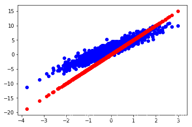
Current loss: 
9.460205

def train(model, inputs, outputs, learning_rate):
  with tf.GradientTape() as t:
    current_loss = loss(model(inputs), outputs)
  dW, db = t.gradient(current_loss, [model.W, model.b])
  model.W.assign_sub(learning_rate * dW)
  model.b.assign_sub(learning_rate * db)

model = Model()

Ws, bs = [], []
epochs = range(10)
for epoch in epochs:
  Ws.append(model.W.numpy())
  bs.append(model.b.numpy())
  current_loss = loss(model(inputs), outputs)

  train(model, inputs, outputs, learning_rate=0.1)
  print('Epoch %2d: W=%1.2f b=%1.2f, loss=%2.5f' %
        (epoch, Ws[-1], bs[-1], current_loss))

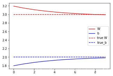
# Let's plot it all
plt.plot(epochs, Ws, 'r',
         epochs, bs, 'b')
plt.plot([TRUE_W] * len(epochs), 'r--',
         [TRUE_b] * len(epochs), 'b--')
plt.legend(['W', 'b', 'true W', 'true_b'])
plt.show()

Epoch  0: W=3.19 b=1.80, loss=1.14858
Epoch  1: W=3.15 b=1.84, loss=1.11297
Epoch  2: W=3.11 b=1.88, loss=1.09001
Epoch  3: W=3.08 b=1.90, loss=1.07521
Epoch  4: W=3.06 b=1.93, loss=1.06567
Epoch  5: W=3.04 b=1.94, loss=1.05952
Epoch  6: W=3.02 b=1.96, loss=1.05555
Epoch  7: W=3.01 b=1.97, loss=1.05300
Epoch  8: W=3.00 b=1.98, loss=1.05135
Epoch  9: W=2.99 b=1.98, loss=1.05028