Up until now, we’ve used only TensorFlow’s high-level API, tf.keras, but it already got us pretty far: we built various neural network architectures, including regression and classification nets, Wide & Deep nets, and self-normalizing nets, using all sorts of techniques, such as Batch Normalization, dropout, and learning rate schedules. In fact, 95% of the use cases you will encounter will not require anything other than tf.keras (and tf.data; see Chapter 13). But now it’s time to dive deeper into TensorFlow and take a look at its lower-level Python API. This will be useful when you need extra control to write custom loss functions, custom metrics, layers, models, initializers, regularizers, weight constraints, and more. You may even need to fully control the training loop itself, for example to apply special transformations or constraints to the gradients (beyond just clipping them) or to use multiple optimizers for different parts of the network. We will cover all these cases in this chapter, and we will also look at how you can boost your custom models and training algorithms using TensorFlow’s automatic graph generation feature. But first, let’s take a quick tour of TensorFlow.
TensorFlow 2.0 (beta) was released in June 2019, making Tensor‐Flow much easier to use. The first edition of this book used TF 1, while this edition uses TF 2.
A Quick Tour of TensorFlow
As you know, TensorFlow is a powerful library for numerical computation, particularly well suited and fine-tuned for large-scale Machine Learning (but you could use it for anything else that requires heavy computations). It was developed by the Google Brain team and it powers many of Google’s large-scale services, such as Google Cloud Speech, Google Photos, and Google Search. It was open sourced in November 2015, and it is now the most popular Deep Learning library (in terms of citations in papers, adoption in companies, stars on GitHub, etc.). Countless projects use TensorFlow for all sorts of Machine Learning tasks, such as image classification, natural language processing, recommender systems, and time series forecasting.
So what does TensorFlow offer? Here’s a summary:
- Its core is very similar to NumPy, but with GPU support.
- It supports distributed computing (across multiple devices and servers).
- It includes a kind of just-in-time (JIT) compiler that allows it to optimize computations for speed and memory usage. It works by extracting the computation graph from a Python function, then optimizing it (e.g., by pruning unused nodes), and finally running it efficiently (e.g., by automatically running independent operations in parallel).
- Computation graphs can be exported to a portable format, so you can train a TensorFlow model in one environment (e.g., using Python on Linux) and run it in another (e.g., using Java on an Android device).
- It implements autodiff (see https://blog.csdn.net/Linli522362242/article/details/106290394 09_Up and Running with TensorFlow_2_Autodiff_momentum optimizer_Mini-batchGradientDescent_SavingMode) and provides some excellent optimizers, such as RMSProp and Nadam (see https://blog.csdn.net/Linli522362242/article/details/106982127 11_Training Deep Neural Networks_2_transfer learning_RBMs_Momentum_Nesterov AccelerG_AdaGrad_RMSProp_Nadam), so you can easily minimize all sorts of loss functions.
TensorFlow offers many more features built on top of these core features: the most important is of course tf.keras,(TensorFlow includes another Deep Learning API called the Estimators API, but the TensorFlow team recommends using tf.keras instead.) but it also has data loading and preprocessing ops (tf.data, tf.io, etc.), image processing ops (tf.image), signal processing ops (tf.signal), and more (see Figure 12-1 for an overview of TensorFlow’s Python API).
We will cover many of the packages and functions of the Tensor‐Flow API, but it’s impossible to cover them all, so you should really take some time to browse through the API; you will find that it is quite rich and well documented.
Figure 12-1. TensorFlow’s Python API
At the lowest level, each TensorFlow operation (op for short) is implemented using highly efficient C++ code.(If you ever need to (but you probably won’t), you can write your own operations using the C++ API.) Many operations have multiple implementations called kernels: each kernel is dedicated to a specific device type, such as CPUs, GPUs, or even TPUs (tensor processing units). As you may know, GPUs can dramatically speed up computations by splitting them into many smaller chunks and running them in parallel across many GPU threads. TPUs are even faster: they are custom ASIC chips built specifically for Deep Learning operations3 (we will discuss how to use TensorFlow with GPUs or TPUs in Chapter 19).
TensorFlow’s architecture is shown in Figure 12-2. Most of the time your code will use the high-level APIs (especially tf.keras and tf.data); but when you need more flexibility, you will use the lower-level Python API, handling tensors directly. Note that APIs for other languages are also available. In any case, TensorFlow’s execution engine will take care of running the operations efficiently, even across multiple devices and machines if you tell it to.
Figure 12-2. TensorFlow’s architecture
TensorFlow runs not only on Windows, Linux, and macOS, but also on mobile devices (using TensorFlow Lite), including both iOS and Android (see Chapter 19). If you do not want to use the Python API, there are C++, Java, Go, and Swift APIs. There is even a JavaScript implementation called TensorFlow.js that makes it possible to run your models directly in your browser.
There’s more to TensorFlow than the library. TensorFlow is at the center of an extensive ecosystem of libraries. First, there’s TensorBoard for visualization (see https://blog.csdn.net/Linli522362242/article/details/106582512). Next, there’s TensorFlow Extended (TFX), which is a set of libraries built by Google to productionize生产 TensorFlow projects: it includes tools for data validation, preprocessing, model analysis, and serving (with TF Serving; see Chapter 19). Google’s TensorFlow Hub provides a way to easily download and reuse pretrained neural networks. You can also get many neural network architectures, some of them pretrained, in TensorFlow’s model garden. Check out the TensorFlow Resources and https://github.com/jtoy/awesome-tensorflow for more TensorFlow-based projects. You will find hundreds of TensorFlow projects on GitHub, so it is often easy to find existing code for whatever you are trying to do.
More and more ML papers are released along with their implementations, and sometimes even with pretrained models. Check out https://paperswithcode.com/ to easily find them.
Last but not least, TensorFlow has a dedicated team of passionate and helpful developers, as well as a large community contributing to improving it. To ask technical questions, you should use http://stackoverflow.com/ and tag your question with tensorflow and python. You can file bugs and feature requests through GitHub. For general discussions, join the Google group.
OK, it’s time to start coding!
Using TensorFlow like NumPy
TensorFlow’s API revolves围绕着 around tensors, which flow from operation to operation—hence the name TensorFlow. A tensor is very similar to a NumPy ndarray: it is usually a multidimensional array, but it can also hold a scalar (a simple value, such as 42). These tensors will be important when we create custom cost functions, custom metrics, custom layers, and more, so let’s see how to create and manipulate them.
Tensors and Operations
Tensors
You can create a tensor with tf.constant().
For example, here is a tensor representing a matrix with two rows and three columns of floats:
import tensorflow as tf

tf.constant([[1., 2., 3.],
             [4., 5., 6.]
            ]) # matrix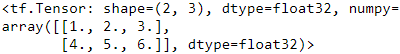
tf.constant(42) #scalar![]()
Just like an ndarray, a tf.Tensor has a shape and a data type (dtype):
t = tf.constant([[1., 2., 3.],
                 [4., 5., 6.]
                ])
t.shape![]()
t.dtype![]()
Indexing works much like in NumPy:
t[:, 1:]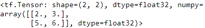
# 如果t是二维数组,t[...,1]等价于t[:,1];如果是三维数值,t[...,1]等价于t[:,:,1]。
# tf.newaxis和np.newaxis功能相同,都是增加维度。
t[..., 1]![]()
t[...,1, tf.newaxis]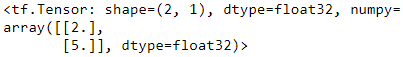
Most importantly, all sorts of tensor operations are available:
t+10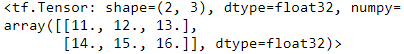
Note that writing t + 10 is equivalent to calling tf.add(t, 10) (indeed, Python calls the magic method t.__add__(10), which just calls tf.add(t, 10)). Other operators like - and * are also supported.
t * 10 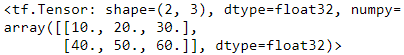
tf.square(t)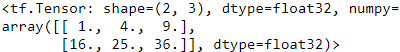
tf.transpose(t)
#t
#[[1., 2., 3.],
# [4., 5., 6.]
#]
t @ tf.transpose(t)
The @ operator was added in Python 3.5, for matrix multiplication: it is equivalent to calling the tf.matmul() function.
You will find all the basic math operations you need (tf.add(), tf.multiply(), tf.square(), tf.exp(), tf.sqrt(), etc.) and most operations that you can find in NumPy (e.g., tf.reshape(), tf.squeeze(), tf.tile()). Some functions have a different name than in NumPy; for instance,
tf.reduce_mean(), tf.reduce_sum(), tf.reduce_max(), and tf.math.log() are the equivalent of
np.mean(), np.sum(), np.max() and np.log(). When the name differs, there is often a good reason for it. For example, in TensorFlow you must write tf.transpose(t); you cannot just write t.T like in NumPy. The reason is that the tf.transpose() function does not do exactly the same thing as NumPy’s T attribute: in TensorFlow, a new tensor is created with its own copy of the transposed data, while in NumPy, t.T is just a transposed view on the same data. Similarly, the tf.reduce_sum() operation is named this way because its GPU kernel (i.e., GPU implementation) uses a reduce algorithm that does not guarantee the order in which the elements are added: because 32-bit floats have limited precision, the result may change ever so slightly every time you call this operation. The same is true of tf.reduce_mean() (but of course tf.reduce_max() is deterministic).
Many functions and classes have aliases. For example, tf.add() and tf.math.add() are the same function. This allows TensorFlow to have concise names for the most common operations while preserving well-organized packages.A notable exception is tf.math.log(), which is commonly used but doesn’t have a tf.log() alias (as it might be confused with logging).
Keras’ Low-Level API
The Keras API has its own low-level API, located in keras.backend. It includes functions like square(), exp(), and sqrt(). In tf.keras, these functions generally just call the corresponding TensorFlow operations. If you want to write code that will be
portable to other Keras implementations, you should use these Keras functions. However, they only cover a subset of all functions available in TensorFlow, so in this book we will use the TensorFlow operations directly. Here is as simple example using keras.backend, which is commonly named K for short:
from tensorflow import keras

K = keras.backend
K.square(K.transpose(t)) + 10
Tensors( tf.constant( ) ) From/To NumPy
Tensors play nice with NumPy: you can create a tensor from a NumPy array, and vice versa. You can even apply TensorFlow operations to NumPy arrays and NumPy operations to tensors:
import numpy as np

a = np.array([2., 4., 5.])
tf.constant(a)![]()
t.numpy()![]()
tf.square(a)![]()
np.square(t)![]()
Notice that NumPy uses 64-bit precision by default, while TensorFlow uses 32-bit. This is because 32-bit precision is generally more than enough for neural networks, plus it runs faster and uses less RAM. So when you create a tensor from a NumPy array, make sure to set dtype=tf.float32.
Type Conversions
Type conversions can significantly hurt performance, and they can easily go unnoticed when they are done automatically. To avoid this, TensorFlow does not perform any type conversions automatically: it just raises an exception if you try to execute an operation on tensors with incompatible types. For example, you cannot add a float tensor and an integer tensor, and you cannot even add a 32-bit float and a 64-bit float:
Conflicting Types
try:
    tf.constant(2.0) + tf.constant(40)
except tf.errors.InvalidArgumentError as ex:
print(ex)![]()
try:#TensorFlow uses 32-bit precision by default
    tf.constant(2.0) + tf.constant(40., dtype=tf.float64)
except tf.errors.InvalidArgumentError as ex:
print(ex)![]()
This may be a bit annoying at first, but remember that it’s for a good cause! And of course you can use tf.cast() when you really need to convert types:
t2 = tf.constant(40., dtype=tf.float64)
tf.constant(2.0) + tf.cast(t2, tf.float32)![]()
Variables
The tf.Tensor values we’ve seen so far are immutable: you cannot modify them. This means that we cannot use regular tensors to implement weights in a neural network, since they need to be tweaked by backpropagation. Plus, other parameters may also need to change over time (e.g., a momentum optimizer keeps track of past gradients). What we need is a tf.Variable:
v = tf.Variable([[1., 2., 3.],
                 [4., 5., 6.]
                ])
v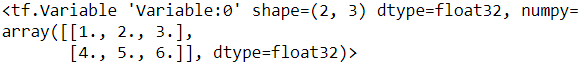
A tf.Variable acts much like a tf.Tensor: you can perform the same operations with it, it plays nicely with NumPy as well, and it is just as picky挑剔的 with types. But it can also be modified in place using the assign() method (or assign_add() or assign_sub(), which increment or decrement the variable by the given value). You can also modify individual cells (or slices), by using the cell’s (or slice’s) assign() method (direct item assignment will not work) or by using the scatter_update() or scatter_nd_update() methods:
v.assign(2*v)
v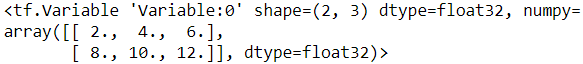
modify individual cells (or slices), by using the cell’s (or slice’s) assign() method
v[0,1].assign(42)
v
<tf.Variable 'Variable:0' shape=(2, 3) dtype=float32, numpy=
array([[ 2., 42., 6.],
[ 8., 10., 12.]], dtype=float32)>v[:,2].assign([0., 1.])
v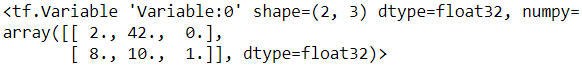
v.scatter_nd_update( indices=[[0,0], [1,2]], updates=[100, 200] )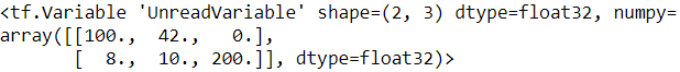
https://www.w3cschool.cn/tensorflow_python/tensorflow_python-g3v22jf1.html
sparse_delta = tf.IndexedSlices( values=[ [1., 2., 3.], [4., 5., 6.] ],
                                 indices=[1,0])
v.scatter_update(sparse_delta)
<tf.Variable 'UnreadVariable' shape=(2, 3) dtype=float32, numpy=
array([[4., 5., 6.],
[1., 2., 3.]], dtype=float32)> In practice you will rarely have to create variables manually, since Keras provides an add_weight() method that will take care of it for you, as we will see. Moreover, model parameters will generally be updated directly by the optimizers, so you will rarely need to update variables manually.
direct item assignment will not work
try:
    v[1] = [7., 8., 9.]
except TypeError as ex:
print(ex) ![]()
Other Data Structures
TensorFlow supports several other data structures, including the following (please see the “Tensors and Operations” section in the notebook or Appendix F for more details):
Tensor arrays (tf.TensorArray)
Are lists of tensors. They have a fixed size by default but can optionally be made dynamic. All tensors they contain must have the same shape and data type.
A tf.TensorArray represents a list of tensors. This can be handy in dynamic models containing loops, to accumulate results and later compute some statistics. You can read or write tensors at any location in the array:
array = tf.TensorArray( dtype=tf.float32, size=3 )
array = array.write( 0, tf.constant([1., 2.]) )
array = array.write( 1, tf.constant([3., 10.]) )
array = array.write( 2, tf.constant([5., 7.]) )

array.read(1)
<tf.Tensor: shape=(2,), dtype=float32, numpy=array([ 3., 10.], dtype=float32)>
Notice that reading an item pops it from the array, replacing it with a tensor of the same shape, full of zeros.
When you write to the array, you must assign the output back to the array, as shown in this code example. If you don’t, although your code will work fine in eager mode, it will break in graph mode (these modes were presented in Chapter 12).
When creating a TensorArray, you must provide its size, except in graph mode. Alternatively, you can leave the size unset and instead set dynamic_size=True, but this will hinder妨碍 performance, so if you know the size in advance, you should set it. You must also specify the dtype, and all elements must have the same shape as the first one written to the array.
You can stack all the items into a regular tensor by calling the stack() method:
array.stack()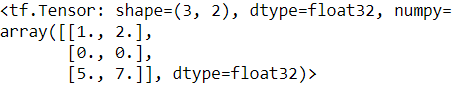
mean, variance = tf.nn.moments( array.stack(), axes=0 )
mean ![]()
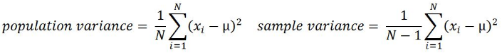
variance ![]()
Ragged tensors (tf.RaggedTensor)
Represent static lists of lists of tensors, where every tensor has the same shape and data type. The tf.ragged package contains operations for ragged tensors.
#p = tf.constant(["Café", "Coffee", "caffè", "咖啡"])
r = tf.strings.unicode_decode(p, "utf8")
r![]()
print(r)![]()
Notice that the decoded strings are stored in a RaggedTensor. What is that?
A ragged tensor is a special kind of tensor that represents a list of arrays of different sizes. More generally, it is a tensor with one or more ragged dimensions, meaning dimensions whose slices may have different lengths. In the ragged tensor r, the second dimension is a ragged dimension. In all ragged tensors, the first dimension is always a regular dimension (also called a uniform dimension).
All the elements of the ragged tensor r are regular tensors. For example, let’s look at the second element of the ragged tensor:
print(r[1])![]()
The tf.ragged package contains several functions to create and manipulate ragged tensors. Let’s create a second ragged tensor using tf.ragged.constant() and concatenate it with the first ragged tensor, along axis 0:
r2 = tf.ragged.constant([ [65,66], [], [67] ])
r2 ![]()
print( tf.concat([r,r2], axis=0) )<tf.RaggedTensor [[67, 97, 102, 233],
[67, 111, 102, 102, 101, 101],
[99, 97, 102, 102, 232],
[21654, 21857],
[65, 66],
[],
[67]]> The result is not too surprising: the tensors in r2 were appended after the tensors in r along axis 0.
But what if we concatenate r and another ragged tensor along axis 1?
r3 = tf.ragged.constant([ [68,69,70], [71], [], [72,73] ])
print(r3)![]()
print( tf.concat([r, r3], axis=1) )<tf.RaggedTensor [[67, 97, 102, 233, 68, 69, 70],
[67, 111, 102, 102, 101, 101, 71],
[99, 97, 102, 102, 232],
[21654, 21857, 72, 73]]>
This time, notice that the tensor in r and the tensor in r3 were concatenated.
Now that’s more unusual, since all of these tensors can have different lengths.
tf.strings.unicode_encode( r3, "UTF-8")<tf.Tensor: shape=(4,), dtype=string, numpy=array([b'DEF', b'G', b'', b'HI'], dtype=object)>
If you call the to_tensor() method, it gets converted to a regular tensor, padding shorter tensors with zeros to get tensors of equal lengths (you can change the default value by setting the default_value argument):
# <tf.RaggedTensor [[67, 97, 102, 233], [67, 111, 102, 102, 101, 101], [99, 97, 102, 102, 232], [21654, 21857]]>
r.to_tensor()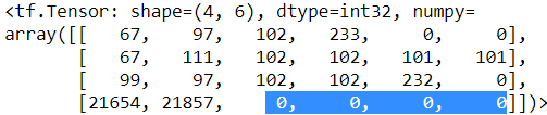
Many TF operations support ragged tensors. For the full list, see the documentation of the tf.RaggedTensor class.
Sparse tensors (tf.SparseTensor)
Efficiently represent tensors containing mostly zeros. The tf.sparse package contains operations for sparse tensors.
TensorFlow can also efficiently represent sparse tensors (i.e., tensors containing mostly zeros). Just create a tf.SparseTensor, specifying the indices and values of the nonzero elements and the tensor’s shape. The indices must be listed in “reading order” (from left to right, and top to bottom). If you are unsure, just use tf.sparse.reorder(). You can convert a sparse tensor to a dense tensor (i.e., a regular tensor) using tf.sparse.to_dense():
s5 = tf.SparseTensor(indices=[[0,2], [0,1]],
                     values=[1., 2.],
                     dense_shape=[3, 4])
print(s5)
SparseTensor(indices=tf.Tensor( [[0 2] [0 1]], shape=(2, 2), dtype=int64),
values=tf.Tensor([1. 2.], shape=(2,), dtype=float32),
dense_shape=tf.Tensor([3 4], shape=(2,), dtype=int64))
try:
    tf.sparse.to_dense(s5)
except tf.errors.InvalidArgumentError as ex:
print(ex) 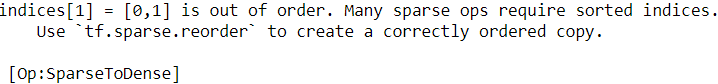
s6 = tf.sparse.reorder(s5)
tf.sparse.to_dense(s6) 
                    # from left to right, and top to bottom
s = tf.SparseTensor( indices= [[0, 1], [1, 0], [2,3]],
                     values = [  1.,     2.,     3.],
                     dense_shape=[3,4])
print(s)
SparseTensor(indices=tf.Tensor([[0 1],[1 0], [2 3]], shape=(3, 2), dtype=int64),
values=tf.Tensor( [1. 2. 3.], shape=(3,), dtype=float32),
dense_shape=tf.Tensor([3 4], shape=(2,), dtype=int64))
tf.sparse.to_dense(s)<tf.Tensor: shape=(3, 4), dtype=float32, numpy=
array([[0., 1., 0., 0.],
[2., 0., 0., 0.],
[0., 0., 0., 3.]], dtype=float32)>
Note that sparse tensors do not support as many operations as dense tensors. For example, you can multiply a sparse tensor by any scalar value, and you get a new sparse tensor, but you cannot add a scalar value to a sparse tensor, as this would not return a sparse tensor:
print(s*3.14)SparseTensor(indices=tf.Tensor([[0 1], [1 0], [2 3]], shape=(3, 2), dtype=int64),
values=tf.Tensor([3.14 6.28 9.42], shape=(3,), dtype=float32),
dense_shape=tf.Tensor([3 4], shape=(2,), dtype=int64))
try:
    s3 = s + 42.0
except TypeError as ex:
print(ex)![]()
s4 = tf.constant([[10., 20.],
                  [30., 40.],
                  [50., 60],
                  [70., 80.]
                 ])
tf.sparse.sparse_dense_matmul(s, s4)
<tf.Tensor: shape=(3, 2), dtype=float32, numpy=
array([[ 30., 40.],
[ 20., 40.],
[210., 240.]], dtype=float32)>
s5 = tf.SparseTensor(indices=[[0,2], [0,2]],
                     values=[1., 2.],
                     dense_shape=[3, 4])
print(s5)
SparseTensor(indices=tf.Tensor( [ [0 2][0 2] ], shape=(2, 2), dtype=int64),
values=tf.Tensor([1. 2.], shape=(2,), dtype=float32),
dense_shape=tf.Tensor([3 4], shape=(2,), dtype=int64))String tensors
Are regular tensors of type tf.string. These represent byte strings, not Unicode strings, so if you create a string tensor using a Unicode string (e.g., a regular Python 3 string like "café"), then it will get encoded to UTF-8 automatically (e.g., b"caf\xc3\xa9"). Alternatively, you can represent Unicode strings using tensors of type tf.int32, where each item represents a Unicode code point (e.g., [99, 97, 102, 233]). The tf.strings package (with an s) contains ops for byte strings and Unicode strings (and to convert one into the other). It’s important to note that a tf.string is atomic, meaning that its length does not appear in the tensor’s shape. Once you convert it to a Unicode tensor (i.e., a tensor of type tf.int32 holding Unicode code points), the length appears in the shape.
tf.constant(b"hello world")![]()
If you try to build a tensor with a Unicode string, TensorFlow automatically encodes it to UTF-8:
tf.constant("café")![]()
It is also possible to create tensors representing Unicode strings. Just create an array of 32-bit integers, each representing a single Unicode code point:
u=tf.constant([ord(c) for c in "café"])# ord('a'):97 # ord('c'):99
u
<tf.Tensor: shape=(4,), dtype=int32, numpy=array([ 99, 97, 102, 233])> However, in a Unicode string tensor (i.e., an int32 tensor), the length of the string is part of the tensor’s shape.
The tf.strings package contains several functions to manipulate string tensors, such as length() to count the number of bytes in a byte string (or the number of code points if you set unit="UTF8_CHAR"), unicode_encode() to convert a Unicode string tensor (i.e., int32 tensor) to a byte string tensor, and unicode_decode() to do the reverse:
b = tf.strings.unicode_encode( u, "UTF-8")
# b : <tf.Tensor: shape=(), dtype=string, numpy=b'caf\xc3\xa9'>
tf.strings.length(b, unit="UTF8_CHAR")![]() # the number of code points
# the number of code points
tf.strings.unicode_decode(b, "UTF-8")![]()
You can also manipulate tensors containing multiple strings:
String arrays
p = tf.constant(["Café", "Coffee", "caffè", "咖啡"])
tf.strings.length(p, unit="UTF8_CHAR") # counted by char![]()
Sets
Are represented as regular tensors (or sparse tensors). For example, tf.constant([ [1, 2], [3, 4] ]) represents the two sets {1, 2} and {3, 4}. More generally, each set is represented by a vector in the tensor’s last axis. You can manipulate sets using operations from the tf.sets package.
TensorFlow supports sets of integers or strings (but not floats). It represents them using regular tensors. For example, the set {1, 5, 9} is just represented as the tensor [[1, 5, 9]]. Note that the tensor must have at least two dimensions, and the sets must be in the last dimension. For example, [[1, 5, 9], [2, 5, 11]] is a tensor holding two independent sets: {1, 5, 9} and {2, 5, 11}. If some sets are shorter than others, you must pad them with a padding value (0 by default, but you can use any other value you prefer).
The tf.sets package contains several functions to manipulate sets. For example, let’s create two sets and compute their union (the result is a sparse tensor, so we call to_dense() to display it):
a = tf.constant([[1,5,9]])
b = tf.constant([[5,6,9,11]])
u = tf.sets.union(a,b)
tf.sparse.to_dense(u)![]()
You can also compute the union of multiple pairs of sets simultaneously:
set1 = tf.constant([ [2,3,5,7], [7,9,0,0] ])
set2 = tf.constant([ [4,5,6], [9,10,0] ])
tf.sparse.to_dense( tf.sets.union(set1, set2) )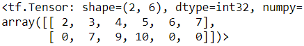
tf.sparse.to_dense( tf.sets.difference(set1, set2) )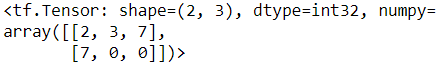
tf.sparse.to_dense( tf.sets.intersection(set1, set2) )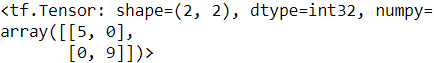
If you prefer to use a different padding value, you must set default_value when calling to_dense():
u = tf.sets.union(set1, set2)
tf.sparse.to_dense( u, default_value=-1)
<tf.Tensor: shape=(2, 6), dtype=int32, numpy=
array([[ 2, 3, 4, 5, 6, 7],
[ 0, 7, 9, 10, -1, -1]])>
The default default_value is 0, so when dealing with string sets, you must set the default_value (e.g., to an empty string).
Queues
Store tensors across multiple steps. TensorFlow offers various kinds of queues: simple First In, First Out (FIFO) queues (FIFOQueue), queues that can prioritize some items (PriorityQueue), shuffle their items (RandomShuffleQueue), and
batch items of different shapes by padding (PaddingFIFOQueue). These classes are all in the tf.queue package.
With tensors, operations, variables, and various data structures at your disposal(自由)处置权, you are now ready to customize your models and training algorithms!
A queue is a data structure to which you can push data records, and later pull them out. TensorFlow implements several types of queues in the tf.queue package. They used to be very important when implementing efficient data loading and preprocessing pipelines, but the tf.data API has essentially rendered them useless无用 (except perhaps in some rare cases) because it is much simpler to use and provides all the tools you need to build efficient pipelines. For the sake of completeness, though, let’s take a quick look at them.
The simplest kind of queue is the first-in, first-out (FIFO) queue. To build it, you need to specify the maximum number of records it can contain. Moreover, each record is a tuple of tensors, so you must specify the type of each tensor, and optionally their shapes.
For example, the following code example creates a FIFO queue with maximum three records, each containing a tuple with a 32-bit integer and a string. Then it pushes two records to it, looks at the size (which is 2 at this point), and pulls a record out:
q = tf.queue.FIFOQueue( 3, [tf.int32, tf.string], shapes=[(), ()] )
q.enqueue([10, b"windy"])
q.enqueue([15, b"sunny"])
q.size()
<tf.Tensor: shape=(), dtype=int32, numpy=2>
q.dequeue() ![]()
It is also possible to enqueue and dequeue multiple records at once (the latter requires specifying the shapes when creating the queue):
q.enqueue_many([ [13, 16], [b'cloudy', b'rainy'] ])
q.dequeue_many(3)
[<tf.Tensor: shape=(3,), dtype=int32, numpy=array([15, 13, 16])>,
<tf.Tensor: shape=(3,), dtype=string, numpy=array([b'sunny', b'cloudy', b'rainy'], dtype=object)>]Other queue types include:
PaddingFIFOQueue
Same as FIFOQueue, but its dequeue_many() method supports dequeueing multiple records of different shapes. It automatically pads the shortest records to ensure all the records in the batch have the same shape.
PriorityQueue
A queue that dequeues records in a prioritized order. The priority must be a 64-bit integer included as the first element of each record. Surprisingly, records with a lower priority will be dequeued first. Records with the same priority will be dequeued in FIFO order.
RandomShuffleQueue
A queue whose records are dequeued in random order. This was useful to implement a shuffle buffer before tf.data existed.
If a queue is already full and you try to enqueue another record, the enqueue*() method will freeze until a record is dequeued by another thread. Similarly, if a queue is empty and you try to dequeue a record, the dequeue*() method will freeze until records are pushed to the queue by another thread.
Customizing Models and Training Algorithms
Let’s start by creating a custom loss function, which is a simple and common use case.
Custom Loss Functions
Suppose you want to train a regression model, but your training set is a bit noisy. Of course, you start by trying to clean up your dataset by removing or fixing the outliers, but that turns out to be insufficient; the dataset is still noisy. Which loss function should you use? The mean squared error might penalize large errors too much and cause your model to be imprecise. The mean absolute error would not penalize outliers as much, but training might take a while to converge, and the trained model might not be very precise. This is probably a good time to use the Huber loss (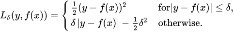 introduced in https://blog.csdn.net/Linli522362242/article/details/106433059, The Huber loss is quadratic when the error is smaller than a threshold δ (typically 1) but linear when the error is larger than δ. The linear part makes it less sensitive to outliers than the mean squared error, and the quadratic part allows it to converge faster and be more precise than the mean absolute error) instead of the good old MSE. The Huber loss is not currently part of the official Keras API, but it is available in tf.keras (just use an instance of the keras.losses.Huber class). But let’s pretend it’s not there: implementing it is easy as pie! Just create a function that takes the labels and predictions as arguments, and use TensorFlow operations to compute every instance’s loss:
Let's start by loading and preparing the California housing dataset. We first load it, then split it into a training set, a validation set and a test set, and finally we scale it:
from sklearn.datasets import fetch_california_housing
from sklearn.model_selection import train_test_split
from sklearn.preprocessing import StandardScaler

housing = fetch_california_housing()
X_train_full, X_test, y_train_full, y_test = train_test_split(
    housing.data, housing.target.reshape(-1, 1), random_state=42
)
X_train, X_valid, y_train, y_valid = train_test_split(
    X_train_full, y_train_full, random_state=42,#If train_size is also None,it will be set to 0.25
)

scaler = StandardScaler()
X_train_scaled = scaler.fit_transform(X_train)
X_valid_scaled = scaler.transform(X_valid)
X_test_scaled = scaler.transform(X_test)

def huber_fn(y_true, y_pred):
    error = y_true-y_pred
    is_small_error = tf.abs(error) < 1 # 1:threshold δ
    squared_loss = tf.square(error)/2
    linear_loss = 1*tf.abs(error) - 0.5*1
    return tf.where(is_small_error, squared_loss, linear_loss)

import matplotlib.pyplot as plt

plt.figure( figsize=(8, 3.5) )
z = np.linspace(-4, 4, 200)
plt.plot(z, huber_fn(0,z), "b-", linewidth=2, label="huber($z$)")
plt.plot(z, z**2/2, "b:", linewidth=1, label=r"$\frac{1}{2}z^2$ when|y-f(x)|<δ")
plt.plot([-1,-1], [0, huber_fn(0., -1.)], "r--")
plt.plot([1,1], [0, huber_fn(0., 1.)], "r--")

plt.gca().axhline(y=0, color="k")
plt.gca().axvline(x=0, color="k")

plt.axis([-4,4, 0,4])
plt.grid(True)
plt.xlabel("$z$")
plt.legend(fontsize=14)
plt.title("Huber loss", fontsize=14)
plt.show()
For better performance, you should use a vectorized implementation, as in this example. Moreover, if you want to benefit from TensorFlow’s graph features, you should use only TensorFlow operations.
It is also preferable to return a tensor containing one loss per instance, rather than returning the mean loss. This way, Keras can apply class weights or sample weights when requested (see https://blog.csdn.net/Linli522362242/article/details/106582512 history.history).
Now you can use this loss when you compile the Keras model, then train your model:
np.random.seed(42)
tf.random.set_seed(42)

input_shape = X_train.shape[1:] # (8,)

model = keras.models.Sequential([
    keras.layers.Dense(30, activation="selu", kernel_initializer="lecun_normal",
                      input_shape = input_shape),
    keras.layers.Dense(1)
])

model.compile( loss=huber_fn, optimizer="nadam", metrics=["mae"])

model.fit(X_train_scaled, y_train, epochs=2, validation_data=(X_valid_scaled, y_valid))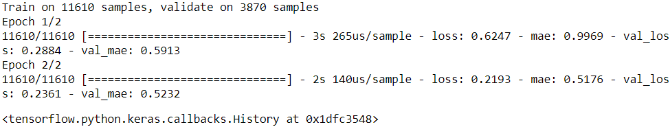
And that’s it! For each batch during training, Keras will call the huber_fn() function to compute the loss and use it to perform a Gradient Descent step. Moreover, it will keep track of the total loss since the beginning of the epoch, and it will display the mean loss.
But what happens to this custom loss when you save the model?
Saving and Loading Models That Contain Custom Components
Saving/Loading Models with Custom Loss Function
Saving a model containing a custom loss function works fine, as Keras saves the name of the function. Whenever you load it, you’ll need to provide a dictionary that maps the function name to the actual function. More generally, when you load a model containing custom objects, you need to map the names to the objects:
model.save("my_model_with_a_custom_loss.h5")
model = keras.models.load_model( "my_model_with_a_custom_loss.h5",
custom_objects={"huber_fn":huber_fn})#############
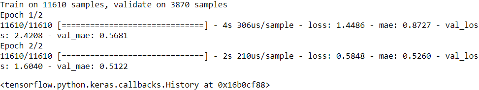
model.fit(X_train_scaled, y_train, epochs=2,
validation_data=(X_valid_scaled, y_valid))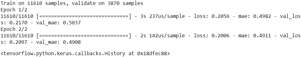
With the current implementation, any error between –1 and 1 is considered “small.” But what if you want a different threshold? One solution is to create a function that creates a configured loss function:
def create_huber(threshold=1.0): #############
    def huber_fn(y_true, y_pred):#############
        error = y_true - y_pred
        is_small_error = tf.abs(error) < threshold
        squared_loss = tf.square(error)/2
        linear_loss = threshold * tf.abs(error) - threshold**2/2
        return tf.where(is_small_error, squared_loss, linear_loss)
    return huber_fn

model.compile(loss=create_huber(2.0), optimizer="nadam", metrics=["mae"]) #############
model.fit(X_train_scaled, y_train, epochs=2, validation_data=(X_valid_scaled, y_valid))
model.save("my_model_with_a_custom_loss_threshold_2.h5")Unfortunately, when you save the model, the threshold will not be saved. This means that you will have to specify the threshold value when loading the model (note that the name to use is "huber_fn", which is the name of the function you gave Keras, not the name of the function that created it):
model = keras.models.load_model("my_model_with_a_custom_loss_threshold_2.h5",
                                custom_objects={"huber_fn":create_huber(2.0)})###
model.fit(X_train_scaled, y_train, epochs=2, validation_data=(X_valid_scaled, y_valid))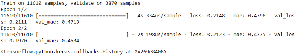
Saving/Loading Models with Custom Loss Subclass
from tensorflow.python.keras.utils import losses_utils

class HuberLoss(keras.losses.Loss):###################
    def __init__(self, threshold=1.0,###################
                 #reduction=losses_utils.ReductionV2.AUTO,
                 name='HuberLoss',
                 **kwargs):
        self.threshold = threshold
        super().__init__(**kwargs)

    def call(self, y_true, y_pred):###################
        error = y_true - y_pred
        is_small_error = tf.abs(error) < self.threshold
        square_loss = tf.square(error)/2
        linear_loss = self.threshold*tf.abs(error) - self.threshold**2/2
        return tf.where( is_small_error, square_loss, linear_loss)

    def get_config(self):###################
        base_config = super().get_config()
#         config={"threshold":self.threshold, 'name':'HuberLoss'}
#         return dict( list(base_config.items()) +
#                      list(config.items())
#                    )
        return {**base_config, "threshold":self.threshold}
np.random.seed(42)
tf.random.set_seed(42)

input_shape = X_train.shape[1:] # (8,)

model = keras.models.Sequential([
    keras.layers.Dense( 30, activation="selu", kernel_initializer="lecun_normal",
                        input_shape=input_shape), #input_shape = X_train.shape[1:] # (8,)
    keras.layers.Dense(1),
])
The Keras API currently only specifies how to use subclassing to define layers, models, callbacks, and regularizers. If you build other components (such as losses, metrics, initializers, or constraints) using subclassing, they may not be portable to other Keras implementations. It’s likely that the Keras API will be updated to specify subclassing for all these components as well.
Let’s walk through this code:
- The constructor accepts **kwargs and passes them to the parent constructor, which handles standard hyperparameters: the name of the loss and the reduction algorithm to use to aggregate the individual instance losses. By default, it is "sum_over_batch_size", which means that the loss will be the sum of the instance losses, weighted by the sample weights, if any, and divided by the batch size (not by the sum of weights, so this is not the weighted mean加权平均值). Other possible values are "sum" and "none".
- The call() method takes the labels and predictions, computes all the instance losses, and returns them.
- The get_config() method returns a dictionary mapping each hyperparameter name to its value. It first calls the parent class’s get_config() method, then adds the new hyperparameters to this dictionary (note that the convenient {**x} syntax was added in Python 3.5).
- You can then use any instance of this class when you compile the model:
model.compile(loss = HuberLoss(2.), optimizer="nadam", metrics=["mae"])
model.fit(X_train_scaled, y_train, epochs=2, validation_data=(X_valid_scaled, y_valid))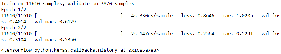
When you save the model, the threshold will be saved along with it; and when you load the model, you just need to map the class name to the class itself:(

 I don't think so)
model.save("my_model_with_a_custom_loss_class.h5")
# When you save the model, the threshold will be saved along with it;
# and when you load the model, you just need to map the class name to the class itself:

model = keras.models.load_model("my_model_with_a_custom_loss_class.h5",
                                custom_objects={"HuberLoss": HuberLoss})

model.fit(X_train_scaled, y_train, epochs=2, validation_data=(X_valid_scaled, y_valid))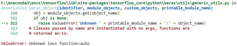
Let's check 'my_model_with_a_custom_loss_class.h5' fileimport h5py f = h5py.File('my_model_with_a_custom_loss_class.h5','r') f.keys()
f['optimizer_weights'].keys()
f['model_weights'].keys()
f.close()So,
# When you save the model, the threshold will be saved along with it;
# and when you load the model, you just need to map the class name to the class itself:
np.random.seed(42)
tf.random.set_seed(42)

model = keras.models.load_model("my_model_with_a_custom_loss_class.h5",
                                custom_objects={"HuberLoss": HuberLoss(2.0)},
                                compile=False
                               )

model.losses
I checked in the TF code and I found the following:
- The function
deserialize_keras_objectfrom generic_utils.py has indeed acustom_objectsargument deserializefrom losses.py has this argument tooget(from losses.py), the function that callsdeserializedoes not fills in this argument- So that, even though I give
custom_objectstoload_modelfunction, it is not passed todeserialize_keras_objectat the end. -
https://github.com/tensorflow/tensorflow/issues/32348
Solution:# When you save the model, the threshold will be saved along with it; # and when you load the model, you just need to map the class name to the class itself: np.random.seed(42) tf.random.set_seed(42) model = keras.models.load_model("my_model_with_a_custom_loss_class.h5", custom_objects={"HuberLoss": HuberLoss(2.0)}, compile=False ) model.compile(loss = HuberLoss(2.0), optimizer="nadam", metrics=["mae"]) model.fit(X_train_scaled, y_train, epochs=2, validation_data=(X_valid_scaled, y_valid))
-
OR
# When you save the model, the threshold will be saved along with it;
# and when you load the model, you just need to map the class name to the class itself:
np.random.seed(42)
tf.random.set_seed(42)

model = keras.models.load_model("my_model_with_a_custom_loss_class.h5",
                                #custom_objects={"HuberLoss": HuberLoss(2.0)},
                                compile=False
                               )
model.compile(loss = HuberLoss(2.0), optimizer="nadam", metrics=["mae"])
model.fit(X_train_scaled, y_train, epochs=2, validation_data=(X_valid_scaled, y_valid))
model.loss.threshold
-
When you save a model, Keras calls the loss instance’s get_config() method and saves the config as JSON in the HDF5 file. When you load the model, it calls the from_config() class method on the HuberLoss class: this method is implemented by the base class (Loss) and creates an instance of the class, passing **config to the constructor.
That’s it for losses! That wasn’t too hard, was it? Just as simple are custom activation functions, initializers, regularizers, and constraints. Let’s look at these now.
Custom Activation Functions, Initializers, Regularizers, and Constraints
Most Keras functionalities, such as losses, regularizers, constraints, initializers, metrics, activation functions, layers, and even full models, can be customized in very much the same way. Most of the time, you will just need to write a simple function
with the appropriate inputs and outputs. Here are examples of a custom activation function (equivalent to keras.activations.softplus() or tf.nn.softplus(), tf.math.log( tf.exp(z)+1.0 )), a custom Glorot initializer (equivalent to keras.initializers.glorot_normal(),Normal distribution with mean 0 and standard deviation 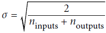 ), a custom ℓ1 regularizer (equivalent to keras.regularizers.l1(0.01)
![]() ), and a custom constraint that ensures weights are all positive (equivalent to keras.constraints.nonneg() or tf.nn.relu()):
), and a custom constraint that ensures weights are all positive (equivalent to keras.constraints.nonneg() or tf.nn.relu()):
import tensorflow as tf
from tensorflow import keras
import numpy as np

keras.backend.clear_session()
np.random.seed(42)
tf.random.set_seed(42)

def my_softplus(z): # return value is just tf.nn.softplus(z)
    return tf.math.log( tf.exp(z)+1.0 )

def my_glorot_initializer(shape, dtype=tf.float32):
    stddev = tf.sqrt( 2. / (shape[0]+shape[1]) )
    return tf.random.normal( shape, stddev=stddev, dtype=dtype )

def my_l1_regularizer(weights):
    return tf.reduce_sum( tf.abs(0.01*weights) )# alpha=0.01 # alpha*sum(weights)

def my_positive_weights(weights): # return value is just tf.nn.relu(weights)
    return tf.where( weights<0., tf.zeros_like(weights), weights )
As you can see, the arguments depend on the type of custom function. These custom functions can then be used normally; for example:
layer = keras.layers.Dense(1,
                           kernel_initializer = my_glorot_initializer, # initialize weights
                           kernel_constraint = my_positive_weights,    ###############
                           kernel_regularizer = my_l1_regularizer,     ###############
                           activation=my_softplus,                     ###############
                          )
The activation function will be applied to the output of this Dense layer, and its result will be passed on to the next layer. The layer’s weights will be initialized using the value returned by the initializer. At each training step the weights will be passed to the regularization function to compute the regularization loss(### for instance,![]() https://blog.csdn.net/Linli522362242/article/details/104124771###), which will be added to the main loss to get the final loss used for training. Finally, the constraint function will be called after each training step, and the layer’s weights will be replaced by the constrained weights.
https://blog.csdn.net/Linli522362242/article/details/104124771###), which will be added to the main loss to get the final loss used for training. Finally, the constraint function will be called after each training step, and the layer’s weights will be replaced by the constrained weights.
keras.backend.clear_session()
np.random.seed(42)
tf.random.set_seed(42)

input_shape = X_train.shape[1:] # (8,)

model = keras.models.Sequential([
    keras.layers.Dense(30, activation = "selu",
                       kernel_initializer = "lecun_normal",
                       input_shape = input_shape),

    keras.layers.Dense(1, activation = my_softplus,###############
                       kernel_initializer = my_glorot_initializer,###############
                       kernel_constraint = my_positive_weights,###############
                       kernel_regularizer= my_l1_regularizer,###############
                      )
])

model.compile(loss="mse", optimizer="nadam", metrics=["mae"])
model.fit(X_train_scaled, y_train, epochs=2,
          validation_data = (X_valid_scaled, y_valid))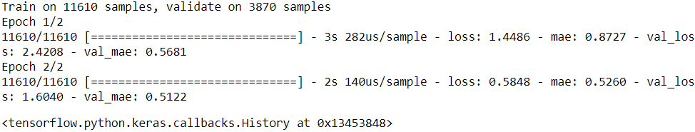
model.save("my_model_with_many_custom_parts.h5")model = keras.models.load_model(
"my_model_with_many_custom_parts.h5",
custom_objects={
'my_softplus' : my_softplus,
'my_glorot_initializer' : my_glorot_initializer,
'my_positive_weights' : my_positive_weights,
'my_l1_regularizer': my_l1_regularizer,
})If a function has hyperparameters that need to be saved along with the model, then you will want to subclass the appropriate class, such as keras.initializers.Initializer, keras.constraints.Constraint, keras.regularizers.Regularizer, or keras.layers.Layer (for any layer, including activation functions). Much like we did for the custom loss, here is a simple class for ℓ1 regularization that saves its factor hyperparameter (this time we do not need to call the parent constructor or the get_config() method, as they are not defined by the parent class):
class MyL1Regularizer( keras.regularizers.Regularizer):###################
    def __init__(self, factor):###################
        self.factor = factor

    def __call__(self, weights):###################
        return tf.reduce_sum( tf.abs(self.factor*weights) ) #L1 norm

    def get_config(self):###################
        return {"factor": self.factor}


keras.backend.clear_session()
np.random.seed(42)
tf.random.set_seed(42)

model = keras.models.Sequential([
    keras.layers.Dense(30, activation="selu", kernel_initializer="lecun_normal",
                       input_shape = input_shape),
    keras.layers.Dense(1, activation=my_softplus,
                       kernel_initializer = my_glorot_initializer,
                       kernel_constraint = my_positive_weights,
                       kernel_regularizer = MyL1Regularizer(0.01),
                      )
])

model.compile( loss="mse", optimizer="nadam", metrics=["mae"])
model.fit(X_train_scaled, y_train, epochs=2,
          validation_data=(X_valid_scaled, y_valid))
Note that you must implement the call() method for losses, layers (including activation functions), and models, or the __call__() method for regularizers, initializers, and constraints. .
model.save("my_model_with_many_custom_parts_MyL1Regularizer.h5")model = keras.models.load_model(
"my_model_with_many_custom_parts_MyL1Regularizer.h5",
custom_objects={
'my_softplus': my_softplus,
'my_glorot_initializer' : my_glorot_initializer,
'my_positive_weights' : my_positive_weights,
'MyL1Regularizer' : MyL1Regularizer,
}
)
model.get_config()
VarianceScaling class https://blog.csdn.net/Linli522362242/article/details/106935910
https://keras.io/api/layers/initializers/
a truncated/untruncated normal distribution with a mean of zero and a standard deviation (after truncation, if used)stddev = sqrt(scale / n), n: number of input units in the weight tensor, if mode="fan_in", here scale=1
{'name': 'sequential',
 'layers': [{'class_name': 'Dense',
   'config': {'name': 'dense',
    'trainable': True,
    'batch_input_shape': (None, 8),
    'dtype': 'float32',
    'units': 30,
    'activation': 'selu',
    'use_bias': True,
    'kernel_initializer': {'class_name': 'VarianceScaling',
     'config': {'scale': 1.0,
      'mode': 'fan_in',
      'distribution': 'truncated_normal',
      'seed': None}},
    'bias_initializer': {'class_name': 'Zeros', 'config': {}},
    'kernel_regularizer': None,
    'bias_regularizer': None,
    'activity_regularizer': None,
    'kernel_constraint': None,
    'bias_constraint': None}},
  {'class_name': 'Dense',
   'config': {'name': 'dense_1',
    'trainable': True,
    'dtype': 'float32',
    'units': 1,
    'activation': 'my_softplus',
    'use_bias': True,
    'kernel_initializer': 'my_glorot_initializer',
    'bias_initializer': {'class_name': 'Zeros', 'config': {}},
    'kernel_regularizer': {'class_name': 'MyL1Regularizer',
     'config': {'factor': 0.01}},
    'bias_regularizer': None,
    'activity_regularizer': None,
    'kernel_constraint': 'my_positive_weights',
    'bias_constraint': None}}]}
For metrics, things are a bit different, as we will see now
Custom Metrics
Losses and metrics are conceptually not the same thing: losses (e.g., cross entropy) are used by Gradient Descent to train a model, so they must be differentiable (at least where they are evaluated), and their gradients should not be 0 everywhere. Plus, it’s OK if they are not easily interpretable by humans. In contrast, metrics (e.g., accuracy) are used to evaluate a model: they must be more easily interpretable, and they can be non-differentiable or have 0 gradients everywhere.
That said, in most cases, defining a custom metric function is exactly the same as defining a custom loss function. In fact, we could even use the Huber loss function we created earlier as a metric###However, the Huber loss is seldom used as a metric (the MAE or MSE is preferred). ###; it would work just fine (and persistence would also work the same way, in this case only saving the name of the function, "huber_fn"):
keras.backend.clear_session()
np.random.seed(42)
tf.random.set_seed(42)

model = keras.models.Sequential([
    keras.layers.Dense(30, activation="selu", kernel_initializer="lecun_normal",
                      input_shape=input_shape),
    keras.layers.Dense(1), #output layer
])

def create_huber(threshold=1.0):
    def huber_fn(y_true, y_pred):
        error = y_true - y_pred
        is_small_error = tf.abs(error) < threshold
        squared_loss = tf.square(error)/2
        linear_loss = threshold * tf.abs(error) - threshold**2/2
        return tf.where(is_small_error, squared_loss, linear_loss)
    return huber_fn

model.compile(loss="mse", optimizer="nadam", metrics=[create_huber(2.0)])

model.fit(X_train_scaled, y_train, epochs=2)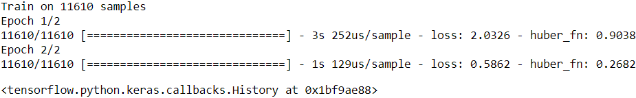
Warning: if you use the same function as the loss and a metric, you may be surprised to see different results. This is generally just due to floating point precision errors: even though the mathematical equations are equivalent, the operations are not run in the same order, which can lead to small differences. Moreover, when using sample weights, there's more than just precision errors:
- the loss since the start of the epoch is the mean of all batch losses seen so far. Each batch loss is the sum of the weighted instance losses divided by the batch size (not the sum of weights, so the batch loss is not the weighted mean of the losses). ### (eg sum( X.shape(batch_size=32,featb ures=8) * W.shape(features, neurons=30) )/ batch size)
- the metric since the start of the epoch is equal to the sum of weighted instance losses divided by sum of all weights seen so far. In other words, it is the weighted mean of all the instance losses. Not the same thing.
### sum( X.shape(batch_size=32,features=8) * W.shape(features, neurons=30) )/ sum of all weights of current batch size
If you do the math, you will find that loss = metric * mean of sample weights (plus some floating point precision error).
https://blog.csdn.net/weixin_40755306/article/details/82290033
sample_weight:权值的numpy array,用于在训练时调整损失函数(仅用于训练)。可以传递一个1D的与样本等长的向量用于对样本进行1对1的加权,或者在面对时序数据时,传递一个的形式为(samples,sequence_length)的矩阵来为每个时间步上的样本赋不同的权。这种情况下请确定在编译模型时添加了sample_weight_mode='temporal'
sample_weigh---主要解决的是样本质量不同的问题,比如前1000个样本的可信度,那么它的权重就要高,后1000个样本可能有错、不可信,那么权重就要调低。
model.compile( loss=create_huber(2.0), optimizer="nadam", metrics=[create_huber(2.0)] )

sample_weight = np.random.rand( len(y_train) ) # len(np.random.rand( len(y_train) ))==len(y_train)
history = model.fit(X_train_scaled, y_train, epochs=2, sample_weight=sample_weight)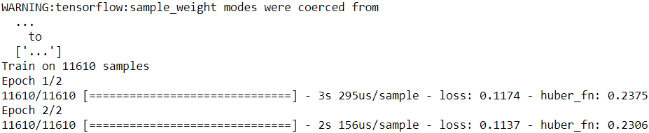
history.history![]()
history.history["loss"][0], history.history["huber_fn"][0]*sample_weight.mean()![]()
Warning: if you use the same function as the loss and a metric, you may be surprised to see different results. This is generally just due to floating point precision errors: even though the mathematical equations are equivalent, the operations are not run in the same order, which can lead to small differences. Moreover, when using sample weights, there's more than just precision errors:
For each batch during training, Keras will compute this metric and keep track of its mean since the beginning of the epoch. Most of the time, this is exactly what you want. But not always! Consider a binary classifier’s precision, for example. As we saw
in Chapter 3, precision is the number of true positives divided by the number of positive predictions (including both true positives and false positives). Suppose the model made five positive predictions in the first batch, four of which were correct(4 true positives and 1 false positives): that’s 80% precision. Then suppose the model made three positive predictions in the second batch, but they were all incorrect( 0 true positives and 3 false positives): that’s 0% precision for the second batch. If you just compute the mean of these two precisions, you get 40%. But wait a second—that’s not the model’s precision over these two batches! Indeed, there were a total of four true positives (4 + 0) out of eight positive predictions (5 + 3), so the overall precision is 50%, not 40%. What we need is an object that can keep track of the number of true
positives and the number of false positives and that can compute their ratio when requested. This is precisely what the keras.metrics.Precision class does:
precision = keras.metrics.Precision()
precision.update_state([0, 1, 1, 1, 0, 1, 0, 1],
                       [1, 1, 0, 1, 0, 1, 0, 1]) #TP(1-->1): 4, #FP(0-->1): 1
#result(): get the current value of the metric
precision.result() #6/8=![]()
# Do not use this statement after previous step if you want to accumulate the result
#precision.reset_states()
precision.update_state([0, 1, 0, 0, 1, 0, 1, 1],
                       [1, 0, 1, 1, 0, 0, 0, 0]) #TP(1-->1): 0, #FP(0-->1): 3
precision.result() #4/(4+1+0+3) ![]()
In this example, we created a Precision object, then we used it like a function, passing it the labels and predictions for the first batch, then for the second batch (note that we could also have passed sample weights). We used the same number of true
and false positives as in the example we just discussed. After the first batch, it returns a precision of 80%; then after the second batch, it returns 50% (which is the overall precision so far, not the second batch’s precision). This is called a streaming metric (or stateful metric), as it is gradually updated, batch after batch.
At any point, we can call the result() method to get the current value of the metric. We can also look at its variables (tracking the number of true and false positives) by using the variables attribute, and we can reset these variables using the reset_states() method:
precision.variables![]()
precision.reset_states() # both variables get reset to 0.0If you need to create such a streaming metric, create a subclass of the keras.metrics.Metric class. Here is a simple example that keeps track of the total Huber loss and the number of instances seen so far. When asked for the result, it returns the ratio, which is simply the mean Huber loss:
from tensorflow import keras

def create_huber(threshold=1.0):
    def huber_fn(y_true, y_pred):
        error = y_true - y_pred
        is_small_error = tf.abs(error) < threshold
        squared_loss = tf.square(error)/2
        linear_loss = threshold * tf.abs(error) - threshold**2/2
        return tf.where(is_small_error, squared_loss, linear_loss)
    return huber_fn

class HuberMetric( keras.metrics.Metric):
    def __init__(self, threshold=1.0, **kwargs):
        super().__init__(**kwargs) # handles base args (e.g., dtype)
        self.threshold = threshold
        self.huber_fn = create_huber( threshold )
        # keeps track of the sum of all Huber losses (total) and
        # the number of instances seen so far (count)
        self.total = self.add_weight("total", initializer="zeros") #tf.Variable
        self.count = self.add_weight("count", initializer="zeros") #tf.Variable

    def update_state(self, y_true, y_pred, sample_weight=None):
        metrics = self.huber_fn(y_true, y_pred) #huber loss
        # modified in place using the assign_add()
        self.total.assign_add(tf.reduce_sum(metrics))# total += sum(metric)
        self.count.assign_add(tf.cast(tf.size(y_true),
                                       tf.float32) )

    def result(self):
        # the update_state() method gets called first,
        # then the result() method is called, and its output is returned
        return self.total / self.count # mean huber loss

    # implement the get_config() method to ensure the threshold
    # gets saved along with the model.
    def get_config(self):
        base_config = super().get_config()
        return {**base_config, "threhold": self.threshold}

    # The default implementation of the reset_states() method resets all variables to 0.0
    # (but you can override it if needed).
Let’s walk through this code:7
- The constructor uses the add_weight() method to create the variables needed to keep track of the metric’s state over multiple batches—in this case, the sum of all Huber losses (total) and the number of instances seen so far (count). You could just create variables manually if you preferred. Keras tracks any tf.Variable that is set as an attribute (and more generally, any “trackable” object, such as layers or models).
- The update_state() method is called when you use an instance of this class as a function (as we did with the Precision object). It updates the variables, given the labels(y_true) and predictions(y_pred) for one batch (and sample weights, but in this case we ignore them).
- The result() method computes and returns the final result, in this case the mean Huber metric over all instances. When you use the metric as a function, the update_state() method gets called first, then the result() method is called, and its output is returned.
- We also implement the get_config() method to ensure the threshold gets saved along with the model.
- The default implementation of the reset_states() method resets all variables to 0.0 (but you can override it if needed).
Warning: when running the following cell, if you get autograph warnings such as WARNING:tensorflow:AutoGraph could not transform [...] and will run it as-is, then please install version 0.2.2 of the gast library (e.g., by running !pip install gast==0.2.2), then restart the kernel and run this notebook again from the beginning (see autograph issue #1 for more details):
import tensorflow as tf
m = HuberMetric(2.0) #threshold=2.0
# total += 2 * |10 - 2| - 2²/2 = 14 since y-f(x)=10-2 > threshold=2.0
# count +=1
# result(mean huber loss) =14/1=14
m(tf.constant([[2.0]]), #y_true
  tf.constant([[10.]])  #y_pred
) ![]()
# total = total + (|1 - 0|² / 2)                          #since y-f(x)=1-0 < threshold=2.0
#               + (2*|9.25 - 5| - 2² /2) =14+ 1/2+6.5 =21 #since y-f(x)=9.25-5 > threshold=2.0
# count = count + 2 = 3
# result = total / count = 21 / 3 = 7
m(tf.constant([[0.], [5.]]),   #y_true OR y
  tf.constant([[1.], [9.25]])) #y_pred OR f(x)

m.result()![]()
m.variables![]()
m.reset_states()
m.variables![]()
Let's check that the HuberMetric class works well:
import numpy as np
input_shape=(8,) #X_train.shape[1:]

keras.backend.clear_session()
np.random.seed(42)
tf.random.set_seed(42)

model = keras.models.Sequential([
    keras.layers.Dense(30, activation="selu", kernel_initializer="lecun_normal",
                      input_shape=input_shape),
    keras.layers.Dense(1)
])
model.compile(loss=create_huber(2.0), optimizer="nadam", metrics=[HuberMetric(2.0)])

# Notice that NumPy uses 64-bit precision by default, while TensorFlow uses 32-bit.
# So when you create a tensor from a NumPy array, make sure to set dtype=tf.float32
model.fit(X_train_scaled.astype(np.float32), y_train.astype(np.float32), epochs=2)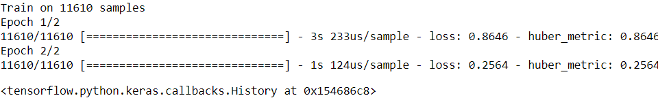
model.save("my_model_with_a_customer_metric.h5")model = keras.models.load_model("my_model_with_a_customer_metric.h5",
custom_objects={"huber_fn": create_huber(2.0),
"HuberMetric": HuberMetric},
# compile=False
)
model.compile(loss=create_huber(2.0), metrics=[HuberMetric(2.0)]) 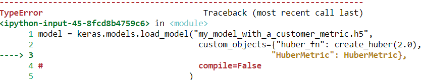
... ...
Solution:
model = keras.models.load_model("my_model_with_a_customer_metric.h5",
#                                 custom_objects={"huber_fn": create_huber(2.0),
#                                                "HuberMetric": HuberMetric},
                                compile=False)
model.compile(loss=create_huber(2.0), metrics=[HuberMetric(2.0)])
model.fit(X_train_scaled.astype(np.float32), y_train.astype(np.float32), epochs=2)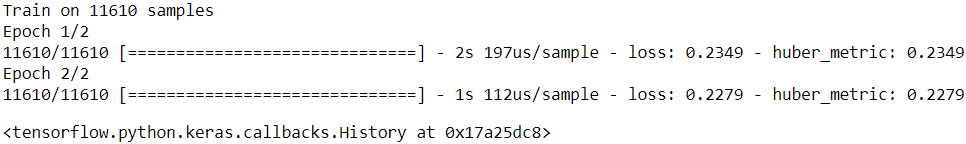
model.metrics_names![]()
Warning: In TF 2.2, tf.keras adds an extra first metric in model.metrics at position 0 (see TF issue #38150 https://github.com/tensorflow/tensorflow/issues/38150). This forces us to use model.metrics[-1] rather than model.metrics[0] to access the HuberMetric.
model.metrics[-1].threshold![]()
Keras will take care of variable persistence seamlessly; no action is required.
When you define a metric using a simple function, Keras automatically calls it for each batch, and it keeps track of the mean during each epoch, just like we did manually. So the only benefit of our HuberMetric class is that the threshold will be saved![]()
![]() . But of course, some metrics, like precision, cannot simply be averaged over batches: in those cases, there’s no other option than to implement a streaming metric.
. But of course, some metrics, like precision, cannot simply be averaged over batches: in those cases, there’s no other option than to implement a streaming metric.
Now that we have built a streaming metric, building a custom layer will seem like a walk in the park!
Custom Layers
You may occasionally want to build an architecture that contains an exotic异国情调 layer for which TensorFlow does not provide a default implementation. In this case, you will need to create a custom layer. Or you may simply want to build a very repetitive architecture, containing identical blocks of layers repeated many times, and it would be convenient to treat each block of layers as a single layer. For example, if the model is a sequence of layers A, B, C, A, B, C, A, B, C, then you might want to define a custom layer D containing layers A, B, C, so your model would then simply be D, D, D. Let’s see how to build custom layers.
First, some layers have no weights, such as keras.layers.Flatten or keras.layers.ReLU. If you want to create a custom layer without any weights, the simplest option is to write a function and wrap it in a keras.layers.Lambda layer. For example, the following layer will apply the exponential function to its inputs:
exponential_layer = keras.layers.Lambda(lambda x: tf.exp(x))
exponential_layer([-1., 0., 1.])
This custom layer can then be used like any other layer, using the Sequential API, the Functional API, or the Subclassing API. You can also use it as an activation function (or you could use activation=tf.exp, activation=keras.activations.exponential, or simply activation="exponential"). The exponential layer is sometimes used in the output layer of a regression model when the values to predict have very different scales (e.g., 0.001, 10., 1,000.).
Adding an exponential layer at the output of a regression model can be useful if the values to predict are positive and with very different scales (e.g., 0.001, 10., 10000):
keras.backend.clear_session()
np.random.seed(42)
tf.random.set_seed(42)
model = keras.models.Sequential([
    keras.layers.Dense(30, activation="relu", input_shape=input_shape),
    keras.layers.Dense(1),
    exponential_layer
])
model.compile(loss="mse", optimizer="nadam")
model.fit(X_train_scaled, y_train, epochs=5,
          validation_data=(X_valid_scaled, y_valid))
model.evaluate( X_test_scaled, y_test ) 
As you’ve probably guessed by now, to build a custom stateful layer (i.e., a layer with weights), you need to create a subclass of the keras.layers.Layer class. For example, the following class implements a simplified version of the Dense layer:
# just for understaing
#inputs, the number of neurons, the name of the layer, the activation function
def neuron_layer( X, n_neurons, name, activation=None):
    with tf.name_scope(name):
        n_inputs = int( X.get_shape()[1] ) # X.get_shape()[1] : the number of features

        stddev = 2 / np.sqrt( n_inputs )
                                       # shape
        init = tf.truncated_normal( (n_inputs, n_neurons), stddev=stddev )
        # truncated_normal( shape, mean=0.0, stdev=1.0 ) # range: [ mean-2*stddev, mean+2*stddev ]
        # stddev=stddev ==> stddev= 2/np.sqrt( n_inputs ) ==> range: mean += 2* 2/np.sqrt( n_inputs )
        # 截断的产生正态分布的随机数,即随机数与均值的差值若大于两倍的标准差,则重新生成 |x-mean| <=2*stddev
        W = tf.Variable(init, name="kernel")
        b = tf.Variable(tf.zeros([n_neurons]), name="bias")
        Z = tf.matmul( X,W) # X dot W # prediction
        if activation is not None:
            return activation(Z)
        else:
            return Z

# https://blog.csdn.net/Linli522362242/article/details/106433059
class MyDense(keras.layers.Layer):
def __init__(self, units, activation=None, **kwargs):
super().__init__(**kwargs)
self.units = units
self.activation = keras.activations.get(activation)
def build(self, batch_input_shape): # batch_input_shape[-1]: features or dimensions
#create connection weights matrix
self.kernel = self.add_weight(
# [n_inputs from previous layer, n_neurons]
name="kernel", shape=[ batch_input_shape[-1], self.units ],
initializer = "glorot_normal") # use it for initializing weight
self.bias = self.add_weight(
name="bias", shape=[self.units], initializer="zeros"
) #trainable=True default
super().build(batch_input_shape) # must be at the end
def call(self, X):
# The @ operator for matrix multiplication
# It is equivalent to calling the tf.matmul() function
# X.shape(batches, features) * W.shape(features, Neurons) + bias.shape(Neurons)
return self.activation( [email protected] + self.bias)
#you can remove it since tf.keras automatically infers the output shape
def compute_output_shape(self, batch_input_shape):
# batch_input_shape.as_list()[:-1] : batches
# self.units : n_neurons
return tf.TensorShape(batch_input_shape.as_list()[:-1] + [self.units])
def get_config(self):
base_config = super().get_config()
return {**base_config,
"units" : self.units,
# Note that we save the activation function’s full configuration by
# calling keras.activations.serialize()
"activation" : keras.activations.serialize(self.activation) }
keras.backend.clear_session()
np.random.seed(42)
tf.random.set_seed(42)
model = keras.models.Sequential([
MyDense(30, activation="relu", input_shape=input_shape),
MyDense(1)
])
model.compile(loss="mse", optimizer="nadam")
model.fit(X_train_scaled, y_train, epochs=2,\
validation_data=(X_valid_scaled, y_valid))
model.evaluate(X_test_scaled, y_test)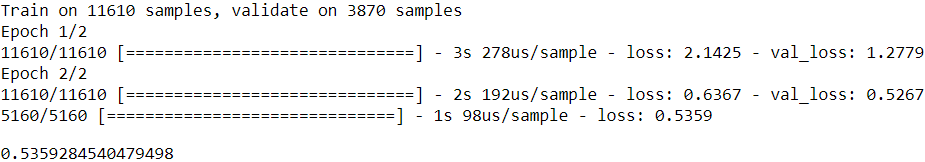
Let’s walk through this code:
- The constructor takes all the hyperparameters as arguments (in this example, units and activation), and importantly it also takes a **kwargs argument. It calls the parent constructor, passing it the kwargs: this takes care of standard arguments such as input_shape, trainable, and name. Then it saves the hyperparameters as attributes, converting the activation argument to the appropriate activation function using the keras.activations.get() function (it accepts functions, standard strings like "relu" or "selu", or simply None).
- The build() method’s role is to create the layer’s variables by calling the add_weight() method for each weight. The build() method is called the first time the layer is used. At that point, Keras will know the shape of this layer’s inputs, and it will pass it to the build() method, which is often necessary to create some of the weights. For example, we need to know the number of neurons in the previous layer in order to create the connection weights matrix (i.e., the "kernel"): this corresponds to the size of the last dimension of the inputs. At the end of the build() method (and only at the end), you must call the parent’s build() method##super().build(batch_input_shape)###: this tells Keras that the layer is built (it just sets self.built=True).
- The call() method performs the desired operations. In this case, we compute the matrix multiplication of the inputs X and the layer’s kernel, we add the bias vector, and we apply the activation function to the result, and this gives us the output of the layer.
- The compute_output_shape() method simply returns the shape of this layer’s outputs. In this case, it is the same shape as the inputs, except the last dimension is replaced with the number of neurons in the layer. Note that in tf.keras, shapes are instances of the tf.TensorShape class, which you can convert to Python lists using as_list().
- The get_config() method is just like in the previous custom classes. Note that we save the activation function’s full configuration by calling keras.activa tions.serialize().
You can now use a MyDense layer just like any other layer!
model.save("my_model_with_a_custom_layer.h5")

model = keras.models.load_model("my_model_with_a_custom_layer.h5",
                                custom_objects={"MyDense":MyDense})
You can generally omit the compute_output_shape() method, as tf.keras automatically infers the output shape, except when the layer is dynamic (as we will see shortly). In other Keras implementations, this method is either required or its default implementation assumes the output shape is the same as the input shape.
To create a layer with multiple inputs (e.g., Concatenate), the argument to the call() method should be a tuple containing all the inputs, and similarly the argument to the compute_output_shape() method should be a tuple containing each input’s batch shape. To create a layer with multiple outputs, the call() method should return the list of outputs, and compute_output_shape() should return the list of batch output shapes (one per output).
For example, the following toy layer takes two inputs and returns three outputs:
class MyMultiLayer( keras.layers.Layer):
    def call(self, X):
        X1, X2 = X
        return X1+X2, X1*X2

    def compute_output_shape(self, batch_input_shape):
        batch_input_shape1, batch_input_shape2 = batch_input_shape
        return [batch_input_shape1, batch_input_shape2]

keras.backend.clear_session()
np.random.seed(42)
tf.random.set_seed(42)

input1 = keras.layers.Input(shape=[2])
input2 = keras.layers.Input(shape=[2])
output1, output2 = MyMultiLayer()((input1, input2))
This layer may now be used like any other layer, but of course only using the Functional and Subclassing APIs, not the Sequential API (which only accepts layers with one input and one output).
If your layer needs to have a different behavior during training and during testing (e.g., if it uses Dropout or BatchNormalization layers), then you must add a training argument to the call() method and use this argument to decide what to do.
For example, let’s create a layer that adds Gaussian noise during training (for regularization) but does nothing during testing (Keras has a layer that does the same thing, keras.layers.GaussianNoise):
class MyGaussianNoise( keras.layers.Layer):
    def __init__(self, stddev, **kwargs):
        super().__init__(**kwargs)
        self.stddev = stddev

    def call(self, X, training=None):
        if training:
            noise = tf.random.normal(tf.shape(X), stddev=self.stddev)
            return X+noise
        else:
            return X

    def compute_output_shape(self, batch_input_shape):
        return batch_input_shape

model.compile(loss="mse", optimizer="nadam")
model.fit(X_train_scaled, y_train, epochs=2,
          validation_data=(X_valid_scaled, y_valid))
model.evaluate(X_test_scaled, y_test)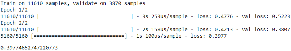
With that, you can now build any custom layer you need! Now let’s create custom models.
Custom Models
We already looked at creating custom model classes in cp10 (https://blog.csdn.net/Linli522362242/article/details/106582512), when we discussed the Subclassing API. It’s straightforward: subclass the keras.Model class, create layers and variables in the constructor, and implement the call() method to do whatever you want the model to do. Suppose you want to build the model represented in Figure 12-3.
Figure 12-3. Custom model example: an arbitrary model with a custom ResidualBlock layer containing a skip connection
The inputs go through a first dense layer, then through a residual block composed of two dense layers and an addition operation (as we will see in Chapter 14, a residual block adds its inputs to its outputs), then through this same residual block three more times, then through a second residual block, and the final result goes through a dense output layer. Note that this model does not make much sense; it’s just an example to illustrate the fact that you can easily build any kind of model you want, even one that contains loops and skip connections. To implement this model, it is best to first create a ResidualBlock layer, since we are going to create a couple of identical blocks (and we might want to reuse it in another model):
class ResidualBlock( keras.layers.Layer ):
    def __init__( self, n_layers, n_neurons, **kwargs):
        super().__init__(**kwargs)
        self.hidden = [keras.layers.Dense(n_neurons, activation="elu",
                                          kernel_initializer="he_normal")
                       for _ in range(n_layers)]

    def call(self, inputs):
        Z = inputs
        for layer in self.hidden:
            Z = layer(Z)
        return inputs + Z # add input to output
This layer is a bit special since it contains other layers. This is handled transparently by Keras: it automatically detects that the hidden attribute contains trackable objects (layers in this case), so their variables are automatically added to this layer’s list of variables. The rest of this class is self-explanatory.
Next, let’s use the Subclassing API to define the model itself:
class ResidualRegressor(keras.Model):
    def __init__(self, output_dim, **kwargs):
        super().__init__(**kwargs)
        self.hidden1 = keras.layers.Dense(30, activation="elu", kernel_initializer="he_normal")
        self.block1 = ResidualBlock(2,30)
        self.block2 = ResidualBlock(2,30)
        self.out = keras.layers.Dense(output_dim)

    def call(self, inputs):
        Z = self.hidden1(inputs)
        for _ in range(1+3):
            Z = self.block1(Z)
        Z = self.block2(Z)
        return self.out(Z)


X_new_scaled = X_test_scaled

keras.backend.clear_session()
np.random.seed(42)
tf.random.set_seed(42)

model = ResidualRegressor(1)
model.compile(loss="mse", optimizer="nadam")
history = model.fit(X_train_scaled, y_train, epochs=5)
score = model.evaluate(X_test_scaled, y_test)
y_pred = model.predict(X_new_scaled)
We create the layers in the constructor and use them in the call() method. This model can then be used like any other model (compile it, fit it, evaluate it, and use it to make predictions). If you also want to be able to save the model using the save() method and load it using the keras.models.load_model() function, you must implement the get_config() method (as we did earlier) in both the ResidualBlock class and the ResidualRegressor class. Alternatively, you can save and load the weights using the save_weights() and load_weights() methods.
model.save("my_custom_model.ckpt")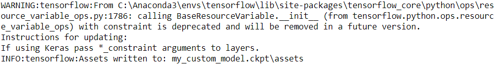
model = keras.models.load_model("my_custom_model.ckpt")

history = model.fit(X_train_scaled, y_train, epochs=5)
The Model class is a subclass of the Layer class, so models can be defined and used exactly like layers. But a model has some extra functionalities, including of course its compile(), fit(), evaluate(), and predict() methods (and a few variants), plus the get_layers() method (which can return any of the model’s layers by name or by index) and the save() method (and support for keras.models.load_model() and keras.models.clone_model()).
If models provide more functionality than layers, why not just define every layer as a model? Well, technically you could, but it is usually cleaner to distinguish the internal components of your model (i.e., layers or reusable blocks of layers) from the model itself (i.e., the object you will train). The former should subclass the Layer class ## class ResidualBlock( keras.layers.Layer ) ##, while the latter should subclass the Model class ## class ResidualRegressor(keras.Model) ##.
We could have defined the model using the sequential API instead:
keras.backend.clear_session()
np.random.seed(42)
tf.random.set_seed(42)

class ResidualBlock( keras.layers.Layer ):
    def __init__( self, n_layers, n_neurons, **kwargs):
        super().__init__(**kwargs)
        self.hidden = [keras.layers.Dense(n_neurons, activation="elu",
                                          kernel_initializer="he_normal")
                       for _ in range(n_layers)]

    def call(self, inputs):
        Z = inputs
        for layer in self.hidden:
            Z = layer(Z)
        return inputs + Z # add input to output

block1 = ResidualBlock(2, 30)
model = keras.models.Sequential([
    keras.layers.Dense(30, activation="elu", kernel_initializer="he_normal"),
    block1, block1, block1, block1,
    ResidualBlock(2,30),
    keras.layers.Dense(1)
])

model.compile(loss="mse", optimizer="nadam")
history = model.fit(X_train_scaled, y_train, epochs=5)
score = model.evaluate(X_test_scaled, y_test)
y_pred = model.predict(X_new_scaled) 
With that, you can naturally and concisely build almost any model that you find in a paper, using the Sequential API, the Functional API, the Subclassing API, or even a mix of these. “Almost” any model? Yes, there are still a few things that we need to look at: first, how to define losses or metrics based on model internals, and second, how to build a custom training loop.
Losses and Metrics Based on Model Internals
The custom losses and metrics we defined earlier were all based on the labels and the predictions (and optionally sample weights). There will be times when you want to define losses based on other parts of your model, such as the weights or activations of its hidden layers. This may be useful for regularization purposes or to monitor some internal aspect of your model.
To define a custom loss based on model internals, compute it based on any part of the model you want, then pass the result to the add_loss() method.For example, let’s build a custom regression MLP model composed of a stack of five hidden layers plus an output layer. This custom model will also have an auxiliary output on top of the upper hidden layer. The loss associated to this auxiliary output will be called the reconstruction loss (see Chapter 17): it is the mean squared difference between the reconstruction and the inputs. By adding this reconstruction loss to the main loss, we will encourage the model to preserve as much information as possible through the hidden layers—even information that is not directly useful for the regression task itself. In practice, this loss sometimes improves generalization (it is a regularization loss). Here is the code for this custom model with a custom reconstruction loss:
class ReconstructingRegressor(keras.Model):
    def __init__(self, output_dim, **kwargs):
        super().__init__(**kwargs)
        self.hidden = [keras.layers.Dense(30, activation="selu",
                                          kernel_initializer="lecun_normal")
                       for _ in range(5)]
        self.out = keras.layers.Dense(output_dim)

    def build(self, batch_input_shape):
        n_inputs = batch_input_shape[-1] #features or dimensions of an instance
        self.reconstruct = keras.layers.Dense(n_inputs)                #########
        # this tells Keras that the layer is built (it just sets self.built=True)
        super().build(batch_input_shape)

    def call(self, inputs, training=None):
        Z = inputs
        for layer in self.hidden:
            Z = layer(Z)
        reconstruction = self.reconstruct(Z)                            ##########
        recon_loss = tf.reduce_mean( tf.square( reconstruction - inputs))#########
        self.add_loss(0.05*recon_loss)                                   #########
        return self.out(Z)


keras.backend.clear_session()
np.random.seed(42)
tf.random.set_seed(42)

model = ReconstructingRegressor(1)
model.compile(loss="mse", optimizer="nadam")
history = model.fit(X_train_scaled, y_train, epochs=2)
y_pred = model.predict(X_test_scaled)
Note: since the number of samples must be divided by batch_size, X_train_scaled[:11584], y_train[:11584] and X_test_scaled[:5152]
Let’s go through this code:
- The constructor creates the DNN with five dense hidden layers and one dense output layer.
- The build() method creates an extra dense layer which will be used to reconstruct the inputs of the model. It must be created here because its number of units must be equal to the number of inputs, and this number is unknown before the build() method is called.
- The call() method processes the inputs through all five hidden layers, then passes the result through the reconstruction layer, which produces the reconstruction.
- Then the call() method computes the reconstruction loss (the mean squared difference between the reconstruction and the inputs), and adds it to the model’s list of losses using the add_loss() method. Notice that we scale down the reconstruction loss by multiplying it by 0.05 (this is a hyperparameter you can tune). This ensures that the reconstruction loss does not dominate the main loss.
- Finally, the call() method passes the output of the hidden layers to the output layer and returns its output.
Similarly, you can add a custom metric based on model internals by computing it in any way you want, as long as the result is the output of a metric object. For example, you can create a keras.metrics.Mean object in the constructor, then call it in the
call() method, passing it the recon_loss, and finally add it to the model by calling the model’s add_metric() method. This way, when you train the model, Keras will display both the mean loss over each epoch (the loss is the sum of the main loss plus
0.05 times the reconstruction loss) and the mean reconstruction error over each epoch. Both will go down during training:
class ReconstructingRegressor(keras.Model):
    def __init__(self, output_dim, **kwargs):
        super().__init__(**kwargs)
        self.hidden = [keras.layers.Dense(30, activation="selu",
                                          kernel_initializer="lecun_normal")
                       for _ in range(5)]
        self.out = keras.layers.Dense(output_dim)
        self.reconstruction_mean = keras.metrics.Mean(name="reconstruction_error")

    def build(self, batch_input_shape):
        n_inputs = batch_input_shape[-1] #features or dimensions of an instance
        self.reconstruct = keras.layers.Dense(n_inputs)                #########
        # this tells Keras that the layer is built (it just sets self.built=True)
        super().build(batch_input_shape)

    def call(self, inputs, training=None):
        Z = inputs
        for layer in self.hidden:
            Z = layer(Z)
        reconstruction = self.reconstruct(Z)                            ##########

        recon_loss = tf.reduce_mean( tf.square( reconstruction - inputs))#########
        self.add_loss(0.05*recon_loss)                                   #########

        if training:
            result = self.reconstruction_mean(recon_loss)
        else:
            result = self.reconstruction_mean(0.)
        self.add_metric(result,name='reconstruction_error', aggregation='mean')

        return self.out(Z)


keras.backend.clear_session()
np.random.seed(42)
tf.random.set_seed(42)

model = ReconstructingRegressor(1)
model.compile(loss="mse", optimizer="nadam")
history = model.fit(X_train_scaled[:11584], y_train[:11584], epochs=2, batch_size=32)
y_pred = model.predict(X_test_scaled[:5152])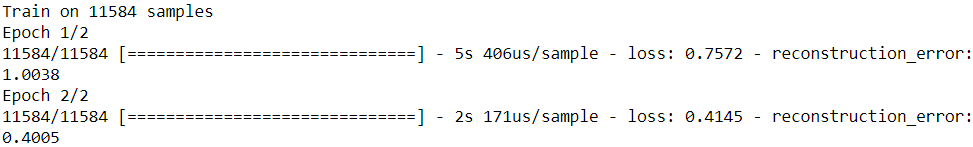
In over 99% of cases, everything we have discussed so far will be sufficient to implement whatever model you want to build, even with complex architectures, losses, and metrics. However, in some rare cases you may need to customize the training loop itself. Before we get there, we need to look at how to compute gradients automatically in TensorFlow.
https://blog.csdn.net/Linli522362242/article/details/107459161