yolov3.py
YOLOv3
输出y_pre
y_pre就是一幅图像图像经过网络之后的输出,内部含有三个特征层的内容: [conv_sbbox, conv_mbbox, conv_lbbox]
三个特征层的shape分别为(N,13,13,255),(N,26,26,255),(N,52,52,255) ?????
def YOLOv3(input_layer):
    route_1, route_2, conv = backbone.darknet53(input_layer)

    conv = common.convolutional(conv, (1, 1, 1024,  512))
    conv = common.convolutional(conv, (3, 3,  512, 1024))
    conv = common.convolutional(conv, (1, 1, 1024,  512))
    conv = common.convolutional(conv, (3, 3,  512, 1024))
    conv = common.convolutional(conv, (1, 1, 1024,  512))

    conv_lobj_branch = common.convolutional(conv, (3, 3, 512, 1024))
    # 第一个输出  最后输出是不加激活也不加BN层
    conv_lbbox = common.convolutional(conv_lobj_branch, (1, 1, 1024, 3*(NUM_CLASS + 5)), activate=False, bn=False)
    conv = common.convolutional(conv, (1, 1,  512,  256))
    conv = common.upsample(conv)
    # 在通道维度上拼接
    conv = tf.concat([conv, route_2], axis=-1)

    conv = common.convolutional(conv, (1, 1, 768, 256))
    conv = common.convolutional(conv, (3, 3, 256, 512))
    conv = common.convolutional(conv, (1, 1, 512, 256))
    conv = common.convolutional(conv, (3, 3, 256, 512))
    conv = common.convolutional(conv, (1, 1, 512, 256))

    conv_mobj_branch = common.convolutional(conv, (3, 3, 256, 512))
    # 第二个输出
    conv_mbbox = common.convolutional(conv_mobj_branch, (1, 1, 512, 3*(NUM_CLASS + 5)), activate=False, bn=False)

    conv = common.convolutional(conv, (1, 1, 256, 128))
    conv = common.upsample(conv)

    conv = tf.concat([conv, route_1], axis=-1)

    conv = common.convolutional(conv, (1, 1, 384, 128))
    conv = common.convolutional(conv, (3, 3, 128, 256))
    conv = common.convolutional(conv, (1, 1, 256, 128))
    conv = common.convolutional(conv, (3, 3, 128, 256))
    conv = common.convolutional(conv, (1, 1, 256, 128))

    conv_sobj_branch = common.convolutional(conv, (3, 3, 128, 256))
    # 第三个输出
    conv_sbbox = common.convolutional(conv_sobj_branch, (1, 1, 256, 3*(NUM_CLASS + 5)), activate=False, bn=False)
    # 我们预测每个尺度上有3个盒子,因此对于4个边界框偏移量,1个对象预测和2个类预测,张量为N×N×[3 *(4 + 1 + 2)]
    return [conv_sbbox, conv_mbbox, conv_lbbox]
decode前:
对于yolo3的模型来说,其最后输出的内容就是三个特征层的内容,三个特征层分别对应着图片被分为不同size的网格后,每个网格点上三个先验框对应的位置、置信度及其种类。
conv_lbbox :tf.Tensor([ 4 76 76 21], shape=(4,), dtype=int32)
conv_mbbox :tf.Tensor([ 4 38 38 21], shape=(4,), dtype=int32)
conv_sbbox :tf.Tensor([ 4 19 19 21], shape=(4,), dtype=int32)
decode后:
对于输出的y1、y2、y3而言,[…, : 2]指的是相对于每个网格点的偏移量,[…, 2: 4]指的是宽和高,[…, 4: 5]指的是该框的置信度,[…, 5: ]指的是每个种类的预测概率。
conv_lbbox :tf.Tensor([ 4 76 76 3 7], shape=(5,), dtype=int32)
conv_mbbox :f.Tensor([ 4 38 38 3 7], shape=(5,), dtype=int32)
conv_sbbox :tf.Tensor([ 4 19 19 3 7], shape=(5,), dtype=int32)
decode
# 3. 利用先验框对网络的输出进行解码(将模型预测参数转化为有物理意义的参数)
def decode(conv_output, i=0):
"""
return tensor of shape [batch_size, output_size, output_size, anchor_per_scale, 5 + num_classes]
contains (x, y, w, h, score, probability)
"""
conv_shape = tf.shape(conv_output)
batch_size = conv_shape[0] # 样本数
output_size = conv_shape[1] # 输出矩阵大小
# 这个reshape为什么能那么恰好地把所有bounding box的5个值都放在矩阵的最里边排列好
conv_output = tf.reshape(conv_output, (batch_size, output_size, output_size, 3, 5 + NUM_CLASS))
# (batch_size, output_size, output_size, 3, 5 + NUM_CLASS) 改为2 + NUM_CLASS
conv_raw_dxdy = conv_output[:, :, :, :, 0:2] # 每个box的tx,ty
conv_raw_dwdh = conv_output[:, :, :, :, 2:4] # 每个box的tw,th
conv_raw_conf = conv_output[:, :, :, :, 4:5] # 置信度
conv_raw_prob = conv_output[:, :, :, :, 5: ] # 类别class 2个 的条件概率
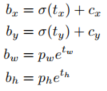
# 将预测值tx,ty,tw,th 通过预测公式的变量关系转化为bounding box中心点坐标以及宽高,bx,by,bh,bw
# 返回 [pred_xywh, pred_conf, pred_prob]
y = tf.tile(tf.range(output_size, dtype=tf.int32)[:, tf.newaxis], [1, output_size])
x = tf.tile(tf.range(output_size, dtype=tf.int32)[tf.newaxis, :], [output_size, 1])
# 若output_size = 5
# x: [[0 1 2 3 4]
# [0 1 2 3 4]
# [0 1 2 3 4]
# [0 1 2 3 4]
# [0 1 2 3 4]]
# y: [[0 0 0 0 0]
# [1 1 1 1 1]
# [2 2 2 2 2]
# [3 3 3 3 3]
# [4 4 4 4 4]]
xy_grid = tf.concat([x[:, :, tf.newaxis], y[:, :, tf.newaxis]], axis=-1)
# x[:, :, tf.newaxis] y[:, :, tf.newaxis]
# [[[0] [[[0]
# [1] [0]
# [2] [0]
# [3] [0]
# [4]] [0]]
# [[0] [[1]
# [1] [1]
# [2] [1]
# [3] [1]
# [4]] [1]]
# [[0] [[2]
# [1] [2]
# [2] [2]
# [3] [2]
# [4]] [2]]
# [[0] [[3]
# [1] [3]
# [2] [3]
# [3] [3]
# [4]] [3]]
# [[0] [[4]
# [1] [4]
# [2] [4]
# [3] [4]
# [4]]] [4]]]
# xy_grid
# [[[0 0]
# [1 0]
# [2 0]
# [3 0]
# [4 0]]
# [[0 1]
# [1 1]
# [2 1]
# [3 1]
# [4 1]]
# [[0 2]
# [1 2]
# [2 2]
# [3 2]
# [4 2]]
# [[0 3]
# [1 3]
# [2 3]
# [3 3]
# [4 3]]
# [[0 4]
# [1 4]
# [2 4]
# [3 4]
# [4 4]]]
xy_grid = tf.tile(xy_grid[tf.newaxis, :, :, tf.newaxis, :], [batch_size, 1, 1, 3, 1])
xy_grid = tf.cast(xy_grid, tf.float32)
# ANCHORS为 3 x 3 个anchor boxes 的长宽
# ANCHORS boxes
# [[[ 1.25 1.625 ]
# [ 2. 3.75 ]
# [ 4.125 2.875 ]]
# [[ 1.875 3.8125 ]
# [ 3.875 2.8125 ]
# [ 3.6875 7.4375 ]]
# [[ 3.625 2.8125 ]
# [ 4.875 6.1875 ]
# [11.65625 10.1875 ]]]
pred_xy = (tf.sigmoid(conv_raw_dxdy) + xy_grid) * STRIDES[i]
pred_wh = (tf.exp(conv_raw_dwdh) * ANCHORS[i]) * STRIDES[i]
pred_xywh = tf.concat([pred_xy, pred_wh], axis=-1)
pred_conf = tf.sigmoid(conv_raw_conf)
pred_prob = tf.sigmoid(conv_raw_prob)
return tf.concat([pred_xywh, pred_conf, pred_prob], axis=-1)
1、tf.shape
tf.shape(
input, out_type=tf.dtypes.int32
)
tf.shape返回表示形状的一维整数张量input。对于标量输入,返回的张量的形状为(0,),其值为空向量(即[])。
t = tf.constant([[[1, 1, 1], [2, 2, 2]], [[3, 3, 3], [4, 4, 4]]])
tf.shape(t)
# <tf.Tensor 'Shape_4:0' shape=(3,) dtype=int32>
2、tf.range
创建一个数字序列。
start = 3
limit = 18
delta = 3
tf.range(start, limit, delta)
# <tf.Tensor 'range:0' shape=(5,) dtype=int32>
参数:
start: 0-D Tensor(标量)。如果limit 不为None,则充当该范围中的第一项;否则,将作为范围限制,并且第一项默认为0。
limit: 0-D Tensor(标量)。序列的上限,不包括在内。如果为None,则默认值为,start而范围的第一项默认为0。
delta:0-D Tensor(标量)。递增的数字start。默认为1。
a = tf.range(output_size,dtype=tf.int32)

b = a[:,tf.newaxis]

c = a[tf.newaxis,:]

sess = tf.Session()

print(sess.run(a))
print(sess.run(b))
print(sess.run(c))
[0 1 2 3 4]
[[0]
 [1]
 [2]
 [3]
 [4]]
[[0 1 2 3 4]]
3、tf.newaxis
给tensor增加维度
a = tf.range(10,dtype=tf.int32)
print(a)
b = a[:,tf.newaxis]
print(b)
# Tensor("range_1:0", shape=(10,), dtype=int32)
# Tensor("strided_slice:0", shape=(10, 1), dtype=int32)
4、tf.cast
将张量转换为新类型。
tf.cast(
x, dtype, name=None
)
x = tf.constant([1.8, 2.2], dtype=tf.float32)
y = tf.dtypes.cast(x, tf.int32)
with tf.Session():
    print(x.eval())
    print(y.eval())
# [1.8 2.2]
# [1 2]
5、tf.title
通过平铺给定张量构造张量。
tf.tile(
    input, multiples, name=None
)
此操作通过复制input multiples次 来创建新的张量
输出张量的第i个维度具有input.dims(i)* multiples [i]元素,并且输入值沿第i个维度重复了multi [i]次。
a = tf.constant([[1,2,3],[4,5,6]], tf.int32)
b = tf.constant([1,2], tf.int32)
c = tf.tile(a, b)
print(sess.run(c))
[[1 2 3 1 2 3]
 [4 5 6 4 5 6]]
a = tf.constant([[1,2,3],[4,5,6]], tf.int32)
b1 = tf.constant([1,2], tf.int32)
out1 = tf.tile(a, b)

b2 = tf.constant([2,1], tf.int32)
out2 = tf.tile(a, b2)

b3 = tf.constant([2,2], tf.int32)
out3 = tf.tile(a, b3)

print(sess.run(out1))
print(sess.run(out2))
print(sess.run(out3))
out1:
[[1 2 3 1 2 3]
 [4 5 6 4 5 6]]
 out2:
[[1 2 3]
 [4 5 6]
 [1 2 3]
 [4 5 6]]
 out3:
[[1 2 3 1 2 3]
 [4 5 6 4 5 6]
 [1 2 3 1 2 3]
 [4 5 6 4 5 6]]
6、tf.concat
沿着某一维度连接张量
tf.concat(
    values, axis, name='concat'
)
t1 = [[1, 2, 3], [4, 5, 6]]
t2 = [[7, 8, 9], [10, 11, 12]]
t3 = tf.concat([t1, t2], 0)
print(sess.run(t3))
[[ 1  2  3]
 [ 4  5  6]
 [ 7  8  9]
 [10 11 12]]
t4 = tf.concat([t1, t2], 1)
print(sess.run(t4))
[[ 1  2  3  7  8  9]
 [ 4  5  6 10 11 12]]
t1 = [[[1, 2], [2, 3]], [[4, 4], [5, 3]]]
t2 = [[[7, 4], [8, 4]], [[2, 10], [15, 11]]]
t3 = tf.concat([t1, t2], -1)
print(sess.run(t3))
[[[ 1  2  7  4]
  [ 2  3  8  4]]

 [[ 4  4  2 10]
  [ 5  3 15 11]]]
7、tf.math.sigmoid
计算 x 元素的 sigmoid
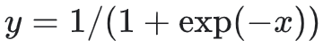
tf.math.sigmoid(
    x
)
8、tf.math.exp
计算x元素的指数

tf.math.exp(
    x
)