动手学深度学习TF2.0第三章

第三章

3.1线性回归

1. 模型定义

这个是线性回归。

2. 模型训练
1训练数据2定义损失函数3优化算法



这里注意小批量随机梯度下降这段话

注意第一句话

3 3.1.2.2 矢量计算表达式
主要介绍了矢量计算的有效性

3.2 线性回归的从零开始实现

%matplotlib inline
import tensorflow as tf
from matplotlib import pyplot as plt
import random


####生成数据集##
num_inputs = 2
num_examples = 1000
true_w = [2, -3.4]
true_b = 4.2
features = tf.random.normal((num_examples, num_inputs),stddev = 1)
##tf.random.normal生成服从正态分布的随机数，第一个参数的python数组，stddev = 1正太分布标准差
labels = true_w[0] * features[:,0] + true_w[1] * features[:,1] + true_b
#这里 true_b是个整数，明显进行了数据的广播机制
labels += tf.random.normal(labels.shape,stddev=0.01)


##按batchsize  读取数据
def data_iter(batch_size, features, labels):
    num_examples = len(features)
    indices = list(range(num_examples))
    random.shuffle(indices)
    for i in range(0, num_examples, batch_size):
        j = indices[i: min(i+batch_size, num_examples)]
        yield tf.gather(features, axis=0, indices=j), tf.gather(labels, axis=0, indices=j)
#tf.gather获取参数的切片第一个为对象，第二个参数为维度，第三个参数为python  数组


###初始化模型参数
w = tf.Variable(tf.random.normal((num_inputs, 1), stddev=0.01))##2行1列
b = tf.Variable(tf.zeros((1,)))

###定义损失函数
def squared_loss(y_hat, y):
    return (y_hat - tf.reshape(y, y_hat.shape)) ** 2 /2
 ##定义模型
def linreg(X, w, b):
    return tf.matmul(X, w) + b

###定义优化算法
def sgd(params, lr, batch_size, grads):
    """Mini-batch stochastic gradient descent."""
    for i, param in enumerate(params):
        param.assign_sub(lr * grads[i] / batch_size)



#训练模型


lr = 0.03
num_epochs = 3
net = linreg
loss = squared_loss
###注意这里调用了tensorflow 的梯度带的语句
for epoch in range(num_epochs):
    for X, y in data_iter(batch_size, features, labels):
        with tf.GradientTape() as t:
            t.watch([w,b])
            l = tf.reduce_sum(loss(net(X, w, b), y))
        grads = t.gradient(l, [w, b])
        sgd([w, b], lr, batch_size, grads)
    train_l = loss(net(features, w, b), labels)
    print('epoch %d, loss %f' % (epoch + 1, tf.reduce_mean(train_l)))

3.3线性回归的简洁实现

这里介绍了TF2.0的keras接口，这里TF2.0版本keras 集成到tensorflow里面。

import tensorflow as tf
#生成数据集
num_inputs = 2
num_examples = 1000
true_w = [2, -3.4]
true_b = 4.2
features = tf.random.normal(shape=(num_examples, num_inputs), stddev=1)
labels = true_w[0] * features[:, 0] + true_w[1] * features[:, 1] + true_b
labels += tf.random.normal(labels.shape, stddev=0.01)


from tensorflow import data as tfdata

batch_size = 10
# 将训练数据的特征和标签组合
dataset = tfdata.Dataset.from_tensor_slices((features, labels))
# 随机读取小批量
dataset = dataset.shuffle(buffer_size=num_examples) 
dataset = dataset.batch(batch_size)
data_iter = iter(dataset)



#定义模型初始化参数
from tensorflow import keras
from tensorflow.keras import layers
from tensorflow import initializers as init
model = keras.Sequential()
model.add(layers.Dense(1, kernel_initializer=init.RandomNormal(stddev=0.01)))

#定义损失函数
from tensorflow import losses
loss = losses.MeanSquaredError()


#定义优化算法
from tensorflow.keras import optimizers
trainer = optimizers.SGD(learning_rate=0.03)

#训练模型
num_epochs = 3
for epoch in range(1, num_epochs + 1):
    for (batch, (X, y)) in enumerate(dataset):
        with tf.GradientTape() as tape:
            l = loss(model(X, training=True), y)

        grads = tape.gradient(l, model.trainable_variables)
        trainer.apply_gradients(zip(grads, model.trainable_variables))

    l = loss(model(features), labels)
    print('epoch %d, loss: %f' % (epoch, l))

3.4 softmax回归

3.6softmax回归的从零开始实现

from tensorflow.keras.datasets import fashion_mnist
import tensorflow as tf
import numpy as np


batch_size=256
(x_train, y_train), (x_test, y_test) = fashion_mnist.load_data()
x_train = tf.cast(x_train, tf.float32) / 255 #在进行矩阵相乘时需要float型，故强制类型转换为float型
x_test = tf.cast(x_test,tf.float32) / 255 #在进行矩阵相乘时需要float型，故强制类型转换为float型
train_iter = tf.data.Dataset.from_tensor_slices((x_train, y_train)).batch(batch_size)
test_iter = tf.data.Dataset.from_tensor_slices((x_test, y_test)).batch(batch_size)



num_inputs = 784
num_outputs = 10
W = tf.Variable(tf.random.normal(shape=(num_inputs, num_outputs), mean=0, stddev=0.01, dtype=tf.float32))
b = tf.Variable(tf.zeros(num_outputs, dtype=tf.float32))



X = tf.constant([[1, 2, 3], [4, 5, 6]])
tf.reduce_sum(X, axis=0, keepdims=True), tf.reduce_sum(X, axis=1, keepdims=True)



def softmax(logits, axis=-1):
    return tf.exp(logits)/tf.reduce_sum(tf.exp(logits), axis, keepdims=True)

def net(X):
    logits = tf.matmul(tf.reshape(X, shape=(-1, W.shape[0])), W) + b
    return softmax(logits)


y_hat = np.array([[0.1, 0.3, 0.6], [0.3, 0.2, 0.5]])
y = np.array([0, 2], dtype='int32')
tf.boolean_mask(y_hat, tf.one_hot(y, depth=3))



def cross_entropy(y_hat, y):
    y = tf.cast(tf.reshape(y, shape=[-1, 1]),dtype=tf.int32)
    y = tf.one_hot(y, depth=y_hat.shape[-1])
    y = tf.cast(tf.reshape(y, shape=[-1, y_hat.shape[-1]]),dtype=tf.int32)
    return -tf.math.log(tf.boolean_mask(y_hat, y)+1e-8)



def accuracy(y_hat, y):
    return np.mean((tf.argmax(y_hat, axis=1) == y))
def evaluate_accuracy(data_iter, net):
    acc_sum, n = 0.0, 0
    for _, (X, y) in enumerate(data_iter):
        y = tf.cast(y,dtype=tf.int64)
        acc_sum += np.sum(tf.cast(tf.argmax(net(X), axis=1), dtype=tf.int64) == y)
        n += y.shape[0]
    return acc_sum / n

num_epochs, lr = 5, 0.1
# 本函数已保存在d2lzh包中方便以后使用
def train_ch3(net, train_iter, test_iter, loss, num_epochs, batch_size, params=None, lr=None, trainer=None):
    for epoch in range(num_epochs):
        train_l_sum, train_acc_sum, n = 0.0, 0.0, 0
        for X, y in train_iter:
            with tf.GradientTape() as tape:
                y_hat = net(X)
                l = tf.reduce_sum(loss(y_hat, y))
            grads = tape.gradient(l, params)
            if trainer is None:
                # 如果没有传入优化器，则使用原先编写的小批量随机梯度下降
                for i, param in enumerate(params):
                    param.assign_sub(lr * grads[i] / batch_size)
            else:
                # tf.keras.optimizers.SGD 直接使用是随机梯度下降 theta(t+1) = theta(t) - learning_rate * gradient
                # 这里使用批量梯度下降，需要对梯度除以 batch_size, 对应原书代码的 trainer.step(batch_size)
                trainer.apply_gradients(zip([grad / batch_size for grad in grads], params))

            y = tf.cast(y, dtype=tf.float32)
            train_l_sum += l.numpy()
            train_acc_sum += tf.reduce_sum(tf.cast(tf.argmax(y_hat, axis=1) == tf.cast(y, dtype=tf.int64), dtype=tf.int64)).numpy()
            n += y.shape[0]
        test_acc = evaluate_accuracy(test_iter, net)
        print('epoch %d, loss %.4f, train acc %.3f, test acc %.3f'% (epoch + 1, train_l_sum / n, train_acc_sum / n, test_acc))

trainer = tf.keras.optimizers.SGD(lr)
train_ch3(net, train_iter, test_iter, cross_entropy, num_epochs, batch_size, [W, b], lr)

预测

import matplotlib.pyplot as plt
X, y = iter(test_iter).next()

def get_fashion_mnist_labels(labels):
    text_labels = ['t-shirt', 'trouser', 'pullover', 'dress', 'coat', 'sandal', 'shirt', 'sneaker', 'bag', 'ankle boot']
    return [text_labels[int(i)] for i in labels]

def show_fashion_mnist(images, labels):
    # 这⾥的_表示我们忽略（不使⽤）的变量
    _, figs = plt.subplots(1, len(images), figsize=(12, 12)) # 这里注意subplot 和subplots 的区别
    for f, img, lbl in zip(figs, images, labels):
        f.imshow(tf.reshape(img, shape=(28, 28)).numpy())
        f.set_title(lbl)
        f.axes.get_xaxis().set_visible(False)
        f.axes.get_yaxis().set_visible(False)
    plt.show()

true_labels = get_fashion_mnist_labels(y.numpy())
pred_labels = get_fashion_mnist_labels(tf.argmax(net(X), axis=1).numpy())
titles = [true + '\n' + pred for true, pred in zip(true_labels, pred_labels)]

show_fashion_mnist(X[0:9], titles[0:9])

3.7softmax回归的简洁实现

import tensorflow as tf
from tensorflow import keras
fashion_mnist = keras.datasets.fashion_mnist
(x_train, y_train), (x_test, y_test) = fashion_mnist.load_data()

x_train = x_train / 255.0
x_test = x_test / 255.0


model = keras.Sequential([
    keras.layers.Flatten(input_shape=(28, 28)),
    keras.layers.Dense(10, activation=tf.nn.softmax)
])

loss = 'sparse_categorical_crossentropy'

optimizer = tf.keras.optimizers.SGD(0.1)

model.compile(optimizer=tf.keras.optimizers.SGD(0.1),
              loss = 'sparse_categorical_crossentropy',
              metrics=['accuracy'])

model.fit(x_train,y_train,epochs=5,batch_size=256)

3.8 多层感知机

如何画一个RELU函数
我用的是pycharm，对代码进行了修改

import tensorflow as tf
from matplotlib import pyplot as plt
import numpy as np
import random

def set_figsize(figsize=(3.5, 2.5)):

    # 设置图的尺寸
    plt.rcParams['figure.figsize'] = figsize

def xyplot(x_vals, y_vals, name):
    set_figsize(figsize=(5, 2.5))
    plt.plot(x_vals.numpy(), y_vals.numpy())
    plt.xlabel('x')
    plt.ylabel(name + '(x)')
x = tf.Variable(tf.range(-8,8,0.1),dtype=tf.float32)
y = tf.nn.relu(x)
xyplot(x, y, 'relu')
plt.show()

画它的导数

with tf.GradientTape() as t:
    t.watch(x)
    y=y = tf.nn.relu(x)
dy_dx = t.gradient(y, x)
xyplot(x, dy_dx, 'grad of relu')
plot.show()

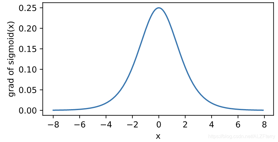
sigmoid

y = tf.nn.sigmoid(x)
xyplot(x, y, 'sigmoid')

依据链式法则，sigmoid函数的导数

扫描二维码关注公众号，回复： 12968198 查看本文章

with tf.GradientTape() as t:
    t.watch(x)
    y=y = tf.nn.sigmoid(x)
dy_dx = t.gradient(y, x)
xyplot(x, dy_dx, 'grad of sigmoid')

3.9 多层感知机的从零开始实现

这里其实就是个例子，怎么自己设计RELU函数，sigmoid函数

import tensorflow as tf
import numpy as np
import sys
sys.path.append("..") # 为了导入上层目录的d2lzh_tensorflow
import d2lzh_tensorflow2 as d2l
from tensorflow.keras.datasets import fashion_mnist
(x_train, y_train), (x_test, y_test) = fashion_mnist.load_data()
batch_size = 256
x_train = tf.cast(x_train, tf.float32)
x_test = tf.cast(x_test, tf.float32)
x_train = x_train/255.0
x_test = x_test/255.0
train_iter = tf.data.Dataset.from_tensor_slices((x_train, y_train)).batch(batch_size)
test_iter = tf.data.Dataset.from_tensor_slices((x_test, y_test)).batch(batch_size)


num_inputs, num_outputs, num_hiddens = 784, 10, 256
W1 = tf.Variable(tf.random.normal(shape=(num_inputs, num_hiddens),mean=0, stddev=0.01, dtype=tf.float32))
b1 = tf.Variable(tf.zeros(num_hiddens, dtype=tf.float32))
W2 = tf.Variable(tf.random.normal(shape=(num_hiddens, num_outputs),mean=0, stddev=0.01, dtype=tf.float32))
b2 = tf.Variable(tf.random.normal([num_outputs], stddev=0.1))

def relu(x):
    return tf.math.maximum(x,0)

def net(X):
    X = tf.reshape(X, shape=[-1, num_inputs])
    h = relu(tf.matmul(X, W1) + b1)
    return tf.math.softmax(tf.matmul(h, W2) + b2)
def loss(y_hat,y_true):
    return tf.losses.sparse_categorical_crossentropy(y_true,y_hat)
num_epochs, lr = 5, 0.5
params = [W1, b1, W2, b2]
d2l.train_ch3(net, train_iter, test_iter, loss, num_epochs, batch_size, params, lr)#与前面的函数

3.12

这一节提到了，为了防止过拟合，使用L2正则化去减少参数的大小。

3.13

应对过拟合的另一个方法
Dropout 丢弃法

Dropout 的目的是防止过分依赖某个参数。
这里值得注意的是，我们只在训练模型的时候使用丢弃法，在测试模型的时候，我们为了得到准确的结果我们并不使用丢弃法。

3.15

回顾3.8节（多层感知机）图3.3描述的多层感知机。为了方便解释，假设输出层只保留一个输出单元，且隐藏层使用相同的激活函数。如果将每个隐藏单元的参数都初始化为相等的值，那么在正向传播时每个隐藏单元将根据相同的输入计算出相同的值，并传递至输出层。在反向传播中，每个隐藏单元的参数梯度值相等。因此，这些参数在使用基于梯度的优化算法迭代后值依然相等。之后的迭代也是如此。在这种情况下，无论隐藏单元有多少，隐藏层本质上只有1个隐藏单元在发挥作用。
因此，正如在前面的实验中所做的那样，我们通常将神经网络的模型参数，特别是权重参数，进行随机初始化。