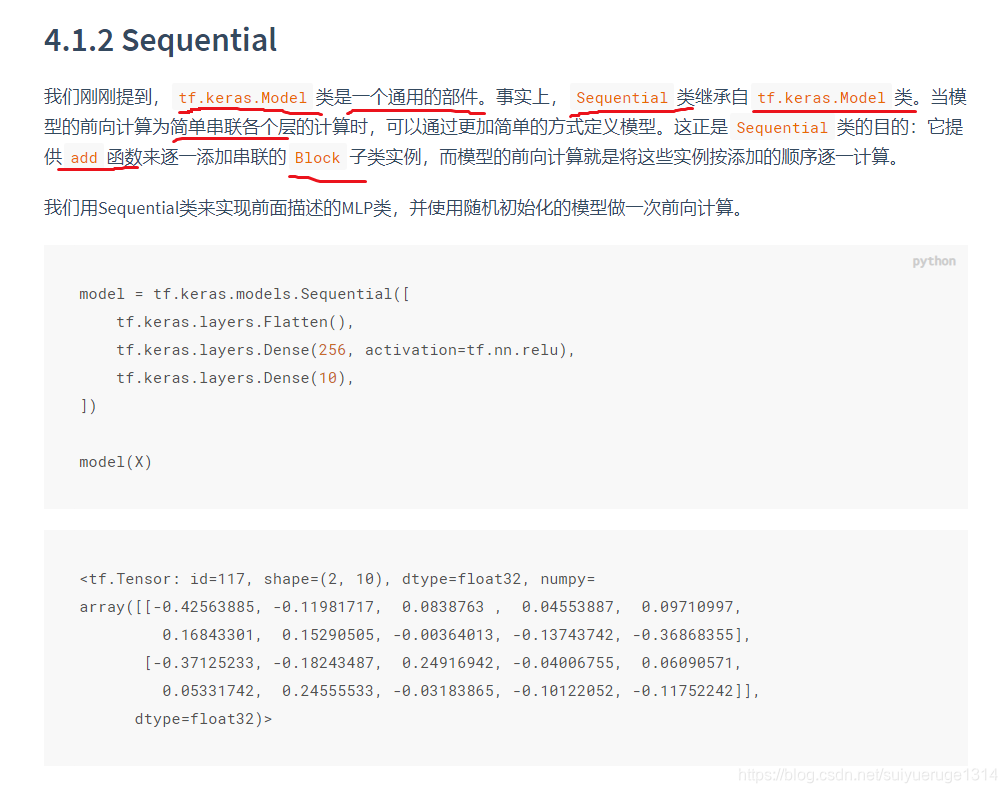
让我们回顾一下在 3.10节(“多层感知机的简洁实现”)一节中含单隐藏层的多层感知机的实现方法。我们首先构造Sequential实例,然后依次添加两个全连接层。其中第一层的输出大小为256,即隐藏层单元个数是256;第二层的输出大小为10,即输出层单元个数是10。我们在上一章的其他 节中也使用了Sequential类构造模型。这里我们介绍另外一种基于tf.keras.Model类的模型构造方法:它让模型构造更加灵活。
两个关键函数:
__init__ 函数
call 函数
import tensorflow as tf
import numpy as np
print(tf.__version__)
class MLP(tf.keras.Model):
    def __init__(self):
        super().__init__()
        self.flatten = tf.keras.layers.Flatten()    # Flatten层将除第一维(batch_size)以外的维度展平
        self.dense1 = tf.keras.layers.Dense(units=256, activation=tf.nn.relu)
        self.dense2 = tf.keras.layers.Dense(units=10)

    def call(self, inputs):
        x = self.flatten(inputs)
        x = self.dense1(x)
        output = self.dense2(x)
        return output
以上的MLP类中无须定义反向传播函数。系统将通过自动求梯度而自动生成反向传播所需的backward函数。
我们可以实例化MLP类得到模型变量net。下面的代码初始化net并传入输入数据X做一次前向计算。其中,net(X)将调用MLP类定义的call函数来完成前向计算。
X = tf.random.uniform((2,20))
net = MLP()
net(X)
#######

<tf.Tensor: id=62, shape=(2, 10), dtype=float32, numpy=
array([[ 0.15637134,  0.14062534, -0.11187253, -0.13151687,  0.12066578,
         0.15376692,  0.03429577,  0.07023033, -0.12030508, -0.38496107],
       [-0.02877349,  0.1088542 , -0.20668823,  0.08241277,  0.06292161,
         0.25310248,  0.04884301,  0.27015388, -0.13183925, -0.23431192]],
      dtype=float32)>

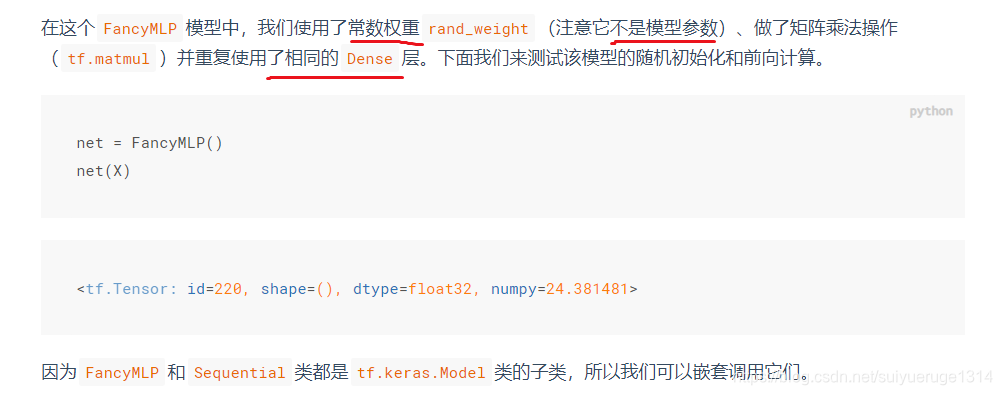
# 构造一个复杂点的模型
class FancyMLP(tf.keras.Model):
    def __init__(self):
        super().__init__()
        self.flatten = tf.keras.layers.Flatten()
        self.rand_weight = tf.constant(
            tf.random.uniform((20,20)))
        self.dense = tf.keras.layers.Dense(units=20, activation=tf.nn.relu)

    def call(self, inputs):
        x = self.flatten(inputs)
        x = tf.nn.relu(tf.matmul(x, self.rand_weight) + 1)
        x = self.dense(x)
        x = tf.nn.relu(tf.matmul(x, self.rand_weight) + 1)
        x = self.dense(x)
        while tf.norm(x) > 1:
            x /= 2
        if tf.norm(x) < 0.8:
            x *= 10
        return tf.reduce_sum(x)