introduction:
python对于常微分方程的数值求解是基于一阶方程进行的,高阶微分方程必须化成一阶方程组,通常采用龙格-库塔方法. scipy.integrate模块的odeint模块的odeint函数求常微分方程的数值解,其基本调用格式为:
sol=odeint(func,y0,t)
func是定义微分方程的函数或匿名函数
y0是初始条件的序列
t是一个自变量取值的序列(t的第一个元素一定必须是初始时刻)
返回值sol是对应于序列t中元素的数值解,如果微分方程组中有n个函数,返回值会是n列的矩阵,第i(i=1,2···,n)列对应于第i个函数的数值解.
其使用的方法和栗子我们可以查看官方给的栗子:
Examples
--------
The second order differential equation for the angle `theta` of a
pendulum acted on by gravity with friction can be written::

    theta''(t) + b*theta'(t) + c*sin(theta(t)) = 0

where `b` and `c` are positive constants, and a prime (') denotes a
derivative.  To solve this equation with `odeint`, we must first convert
it to a system of first order equations.  By defining the angular
velocity ``omega(t) = theta'(t)``, we obtain the system::

    theta'(t) = omega(t)
    omega'(t) = -b*omega(t) - c*sin(theta(t))

Let `y` be the vector [`theta`, `omega`].  We implement this system
in python as:

>>> def pend(y, t, b, c):
...     theta, omega = y
...     dydt = [omega, -b*omega - c*np.sin(theta)]
...     return dydt
...

We assume the constants are `b` = 0.25 and `c` = 5.0:

>>> b = 0.25
>>> c = 5.0

For initial conditions, we assume the pendulum is nearly vertical
with `theta(0)` = `pi` - 0.1, and is initially at rest, so
`omega(0)` = 0.  Then the vector of initial conditions is

>>> y0 = [np.pi - 0.1, 0.0]

We will generate a solution at 101 evenly spaced samples in the interval
0 <= `t` <= 10.  So our array of times is:

>>> t = np.linspace(0, 10, 101)

Call `odeint` to generate the solution.  To pass the parameters
`b` and `c` to `pend`, we give them to `odeint` using the `args`
argument.

>>> from scipy.integrate import odeint
>>> sol = odeint(pend, y0, t, args=(b, c))

The solution is an array with shape (101, 2).  The first column
is `theta(t)`, and the second is `omega(t)`.  The following code
plots both components.

>>> import matplotlib.pyplot as plt
>>> plt.plot(t, sol[:, 0], 'b', label='theta(t)')
>>> plt.plot(t, sol[:, 1], 'g', label='omega(t)')
>>> plt.legend(loc='best')
>>> plt.xlabel('t')
>>> plt.grid()
>>> plt.show()
"""
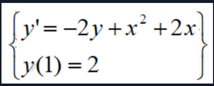
例题1:给定方程,求在1<<x<10步长间隔为0.5 点上的数值解
from scipy.integrate import odeint
from numpy import arange
dy=lambda y,x: -2*y+x**2+2*x
x=arange(1,10.5,0.5)
sol=odeint(dy,2,x)
print("x={}\n对应的数值解y={}".format(x,sol.T))
output:
x=[ 1.   1.5  2.   2.5  3.   3.5  4.   4.5  5.   5.5  6.   6.5  7.   7.5
  8.   8.5  9.   9.5 10. ]
对应的数值解y=[[ 2.          2.08484933  2.9191691   4.18723381  5.77289452  7.63342241
   9.75309843 12.12613985 14.75041934 17.62515427 20.75005673 24.12502089
  27.7500077  31.62500278 35.75000104 40.1250004  44.75000015 49.62500006
  54.75000002]]
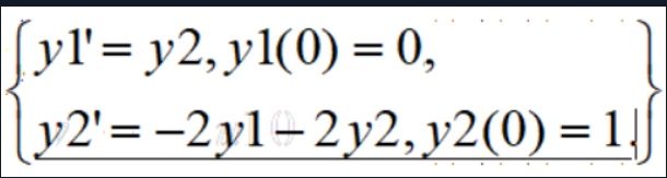
例题2:求上述方程的数值解,并在同一个图形界面上画出符号解和数值解的曲线

引进y1=y,y2=y’,则可以把原来的二阶微分方程(在该方程中出现因变量的二阶导数,我们就称为二阶(常)微分方程)化为如下一阶微分方程组:
from scipy.integrate import odeint
from sympy.abc import t
import numpy as np
import matplotlib.pyplot as plt
#定义一个方程组(微分方程组)
def pfun(y,x):
	y1,y2=y; #让'y'成为一个[y1',y2']的向量 所以将等式左边都化为1阶微分是很重要的
	return np.array([y2,-2*y1-2*y2]) #返回的是等式右边的值
x=np.arange(0,10,0.1) #创建自变量序列
soli=odeint(pfun,[0.0,1.0],x) #求数值解
plt.rc('font',size=16); plt.rc('font',family='SimHei')
plt.plot(x,soli[:,0],'r*',label="数值解")
plt.plot(x,np.exp(-x)*np.sin(x),'g',label="符号解曲线")
plt.legend()
plt.show()

例题3: Lorenz的混沌效应
Lorenz模型:
一阶自治常微分方程组(不显含时间变量)

σ ρ β 分 别 是 模 型 的 三 个 参 数 \sigma \rho \beta 分别是模型的三个参数 σρβ分别是模型的三个参数
这里我们对这个方程组进行数值求解 并画出两个图
Figure 1 是Lorenz模型在
σ = 10 ∣ ∣ ρ = 28 ∣ ∣ β = 8 / 3 \sigma=10 || \rho=28 || \beta=8/3 σ=10∣∣ρ=28∣∣β=8/3
条件时系统的三维演化轨迹
Figure2 是系统从两个靠的很近的初值**(在代码中我们定义怕偏差值为0.01)**出发后,解的偏差演化曲线
from scipy.integrate import odeint
import numpy as np
from mpl_toolkits import mplot3d
import matplotlib.pyplot as plt
def lorenz(w,t): #定义微分方程组
	sigma=10;rho=28;beta=8/3
	x,y,z=w
	return np.array([sigma*(y-x),rho*x-y-x*z,x*y-beta*z])
t=np.arange(0,50,0.01) #建立自变量序列(也就是时间点)
sol1=odeint(lorenz, [0.0,1.0,0.0],t) #第一个初值问题求解
sol2=odeint(lorenz,[0.0,1.001,0.0],t) #第二个初值问题求解
#画图代码 (可忽略)
plt.rc('font',size=16); plt.rc('text',usetex=False)
#第一个图的各轴的定义
ax1=plt.subplot(121,projection='3d')
ax1.plot(sol1[:,0],sol1[:,1],sol1[:,2],'r')
ax1.set_xlabel('$x$');ax1.set_ylabel('$y$');ax1.set_zlabel('$z$')
ax2=plt.subplot(122,projection='3d')
ax2.plot(sol1[:,0]-sol2[:,0],sol1[:,1]-sol2[:,1],
		 sol1[:,2]-sol2[:,2],'g')
ax2.set_xlabel('$x$');ax2.set_ylabel('$y$');ax2.set_zlabel('$z$')
plt.show()
print("sol1=",sol1,'\n\n',"sol1-sol2",sol1-sol2)

结论:
由Figure1 可以看出经过长时间运行后,系统只在三维空间的一个有限区域内运动,即在三维相空间里的测度为0
由Figure2 可以看出系统虽然从两个靠的很近的初值出发,但是随着时间的增大,两个解的差异会越来越大