文章目录
一、scara机器人雅克比矩阵
1、雅克比矩阵推导
scara机器人的运动学正解为:
{ x = L 1 c o s θ 1 + L 2 c o s ( θ 1 + θ 2 ) y = L 1 s i n θ 1 + L 2 s i n ( θ 1 + θ 2 ) z = θ 3 s 2 π c = θ 1 + θ 2 + θ 4 (1) \begin{cases} x=L_1cos\theta_1+L_2cos(\theta_1+\theta_2) \\ y=L_1sin\theta_1+L_2sin(\theta_1+\theta_2) \\ z=\frac{\theta_3s}{2\pi} \\ c=\theta_1+ \theta_2+ \theta_4 \tag 1 \end{cases} ⎩⎪⎪⎪⎨⎪⎪⎪⎧x=L1cosθ1+L2cos(θ1+θ2)y=L1sinθ1+L2sin(θ1+θ2)z=2πθ3sc=θ1+θ2+θ4(1)
参考我另一篇博文:scara机器人运动学正逆解。
上式两边对时间 t t t求导,得:
{ v x = − L 1 s i n θ 1 θ 1 ˙ − L 2 s i n ( θ 1 + θ 2 ) ( θ 1 ˙ + θ 2 ˙ ) v y = L 1 c o s θ 1 θ 1 ˙ + L 2 c o s ( θ 1 + θ 2 ) ( θ 1 ˙ + θ 2 ˙ ) v z = θ 3 ˙ s 2 π v c = θ 1 ˙ + θ 2 ˙ + θ 4 ˙ (2) \begin{cases} v_x=-L_1sin\theta_1\dot{\theta_1}-L_2sin(\theta_1+\theta_2)(\dot{\theta_1} + \dot{\theta_2}) \\ v_y=L_1cos\theta_1\dot{\theta_1}+L_2cos(\theta_1+\theta_2) (\dot{\theta_1} + \dot{\theta_2}) \\ v_z=\frac{\dot{\theta_3}s}{2\pi} \\ v_c=\dot{\theta_1}+ \dot{\theta_2}+ \dot{\theta_4} \tag 2 \end{cases} ⎩⎪⎪⎪⎨⎪⎪⎪⎧vx=−L1sinθ1θ1˙−L2sin(θ1+θ2)(θ1˙+θ2˙)vy=L1cosθ1θ1˙+L2cos(θ1+θ2)(θ1˙+θ2˙)vz=2πθ3˙svc=θ1˙+θ2˙+θ4˙(2)
上式写成矩阵形式,得:
[ v x v y v z v c ] = J [ θ 1 ˙ θ 2 ˙ θ 3 ˙ θ 4 ˙ ] (3) \left[ \begin{matrix} v_x \\ v_y \\ v_z \\ v_c \end{matrix} \right] = J \left[ \begin{matrix} \dot{\theta_1} \\ \dot{\theta_2} \\ \dot{\theta_3} \\ \dot{\theta_4} \end{matrix} \right] \tag{3} ⎣⎢⎢⎡vxvyvzvc⎦⎥⎥⎤=J⎣⎢⎢⎡θ1˙θ2˙θ3˙θ4˙⎦⎥⎥⎤(3)
其中 J J J为雅克比矩阵:
J = [ − L 1 s i n θ 1 − L 2 s i n ( θ 1 + θ 2 ) − L 2 s i n ( θ 1 + θ 2 ) 0 0 L 1 c o s θ 1 + L 2 c o s ( θ 1 + θ 2 ) L 2 c o s ( θ 1 + θ 2 ) 0 0 0 0 s / ( 2 π ) 0 1 1 0 1 ] (4) J=\left[ \begin{matrix} -L_1sin\theta_1-L_2sin(\theta_1+\theta_2) & -L_2sin(\theta_1+\theta_2) & 0 & 0\\ L_1cos\theta_1+L_2cos(\theta_1+\theta_2) & L_2cos(\theta_1+\theta_2) & 0 & 0 \\ 0 & 0 & s/(2\pi) & 0 \\ 1 & 1 & 0 & 1 \end{matrix} \right] \tag{4} J=⎣⎢⎢⎡−L1sinθ1−L2sin(θ1+θ2)L1cosθ1+L2cos(θ1+θ2)01−L2sin(θ1+θ2)L2cos(θ1+θ2)0100s/(2π)00001⎦⎥⎥⎤(4)
由式(3)可知,雅克比矩阵是机器人末端速度与关节速度的桥梁,是两者间的映射关系。雅克比矩阵的行列式为:
∣ J ∣ = ∣ − L 1 s i n θ 1 − L 2 s i n ( θ 1 + θ 2 ) − L 2 s i n ( θ 1 + θ 2 ) 0 0 L 1 c o s θ 1 + L 2 c o s ( θ 1 + θ 2 ) L 2 c o s ( θ 1 + θ 2 ) 0 0 0 0 s / ( 2 π ) 0 1 1 0 1 ∣ = L 1 L 2 s 2 π s i n θ 2 (5) \begin{aligned} |J|&=\left| \begin{matrix} -L_1sin\theta_1-L_2sin(\theta_1+\theta_2) & -L_2sin(\theta_1+\theta_2) & 0 & 0\\ L_1cos\theta_1+L_2cos(\theta_1+\theta_2) & L_2cos(\theta_1+\theta_2) & 0 & 0 \\ 0 & 0 & s/(2\pi) & 0 \\ 1 & 1 & 0 & 1 \end{matrix} \right| \\ &= \frac{L_1L_2s}{2\pi}sin{\theta_2} \\ \tag{5} \end{aligned} ∣J∣=∣∣∣∣∣∣∣∣−L1sinθ1−L2sin(θ1+θ2)L1cosθ1+L2cos(θ1+θ2)01−L2sin(θ1+θ2)L2cos(θ1+θ2)0100s/(2π)00001∣∣∣∣∣∣∣∣=2πL1L2ssinθ2(5)
当 s i n θ 2 = 0 sin{\theta_2}=0 sinθ2=0时, ∣ J ∣ = 0 |J|=0 ∣J∣=0,雅克比矩阵不可逆,此时机器人处于奇异位置。在奇异位置,无法通过机器人末端速度和雅克比矩阵计算得到机器人关节速度。或者说,在奇异位置,通过机器人末端速度和雅克比矩阵计算得到的机器人关节速度为无穷大,这在实际物理世界是不可能的。因此,机器人笛卡尔空间插补运动(直线、圆弧、样条插补等)一定要考虑并避开奇异位置。
2、机器人末端速度与关节速度、末端加速度与关节加速度之间相互转换
(1)、已知关节速度,计算末端速度
已知机器人在工作空间内任意位置(即使是奇异位置,即 s i n θ 2 = 0 sin{\theta_2}=0 sinθ2=0)的关节位置和关节速度,通过雅克比矩阵,可以根据式(3)直接求得。
(2)、已知关节加速度,计算末端加速度
式(3)两边对时间t求导,得:
[ a x a y a z a c ] = J ˙ [ θ 1 ˙ θ 2 ˙ θ 3 ˙ θ 4 ˙ ] + J [ θ 1 ¨ θ 2 ¨ θ 3 ¨ θ 4 ¨ ] (6) \left[ \begin{matrix} a_x \\ a_y \\ a_z \\ a_c \end{matrix} \right] = \dot{J} \left[ \begin{matrix} \dot{\theta_1} \\ \dot{\theta_2} \\ \dot{\theta_3} \\ \dot{\theta_4} \end{matrix} \right] +J\left[ \begin{matrix} \ddot{\theta_1} \\ \ddot{\theta_2} \\ \ddot{\theta_3} \\ \ddot{\theta_4} \end{matrix} \right] \tag{6} ⎣⎢⎢⎡axayazac⎦⎥⎥⎤=J˙⎣⎢⎢⎡θ1˙θ2˙θ3˙θ4˙⎦⎥⎥⎤+J⎣⎢⎢⎡θ1¨θ2¨θ3¨θ4¨⎦⎥⎥⎤(6)
其中:
J ˙ = [ − L 1 c o s θ 1 θ 1 ˙ − L 2 c o s ( θ 1 + θ 2 ) ( θ 1 ˙ + θ 2 ˙ ) − L 2 c o s ( θ 1 + θ 2 ) ( θ 1 ˙ + θ 2 ˙ ) 0 0 − L 1 s i n θ 1 θ 1 ˙ − L 2 s i n ( θ 1 + θ 2 ) ( θ 1 ˙ + θ 2 ˙ ) − L 2 s i n ( θ 1 + θ 2 ) ( θ 1 ˙ + θ 2 ˙ ) 0 0 0 0 0 0 0 0 0 0 ] (7) \dot{J}=\left[ \begin{matrix} -L_1cos\theta_1\dot{\theta_1}-L_2cos(\theta_1+\theta_2) (\dot{\theta_1}+\dot{\theta_2}) & -L_2cos(\theta_1+\theta_2)(\dot{\theta_1}+\dot{\theta_2}) & 0 & 0\\ -L_1sin\theta_1\dot{\theta_1}-L_2sin(\theta_1+\theta_2)(\dot{\theta_1}+\dot{\theta_2}) & -L_2sin(\theta_1+\theta_2)(\dot{\theta_1}+\dot{\theta_2}) & 0 & 0 \\ 0 & 0 & 0 & 0 \\ 0 & 0 & 0 & 0 \end{matrix} \right] \tag{7} J˙=⎣⎢⎢⎡−L1cosθ1θ1˙−L2cos(θ1+θ2)(θ1˙+θ2˙)−L1sinθ1θ1˙−L2sin(θ1+θ2)(θ1˙+θ2˙)00−L2cos(θ1+θ2)(θ1˙+θ2˙)−L2sin(θ1+θ2)(θ1˙+θ2˙)0000000000⎦⎥⎥⎤(7)
(3)、已知末端速度,计算关节速度
当机器人不在奇异位置时,根据式(3),关节速度如下计算:
[ θ 1 ˙ θ 2 ˙ θ 3 ˙ θ 4 ˙ ] = J − 1 [ v x v y v z v c ] (8) \left[ \begin{matrix} \dot{\theta_1} \\ \dot{\theta_2} \\ \dot{\theta_3} \\ \dot{\theta_4} \end{matrix} \right] = J^{-1}\left[ \begin{matrix} v_x \\ v_y \\ v_z \\ v_c \end{matrix} \right] \tag{8} ⎣⎢⎢⎡θ1˙θ2˙θ3˙θ4˙⎦⎥⎥⎤=J−1⎣⎢⎢⎡vxvyvzvc⎦⎥⎥⎤(8)
由于3,4轴关节速度很容易根据式(2)单独求得:
{ θ 3 ˙ = 2 π v z / s θ 4 ˙ = v c − θ 1 ˙ − θ 2 ˙ (9) \begin{cases} \dot{\theta_3}=2\pi v_z / s \\ \dot{\theta_4}=v_c-\dot{\theta_1}- \dot{\theta_2} \\ \tag {9} \end{cases} {
θ3˙=2πvz/sθ4˙=vc−θ1˙−θ2˙(9)
只考虑1,2轴关节速度的计算显得更加简单,计算量也更小。令:
{ s 1 = s i n θ 1 s 12 = s i n ( θ 1 + θ 2 ) c 1 = c o s θ 1 c 12 = c o s ( θ 1 + θ 2 ) (10) \begin{cases} s_1=sin\theta_1 \\ s_{12}=sin(\theta_1+\theta_2) \\ c_1=cos\theta_1 \\ c_{12}=cos(\theta_1+\theta_2) \tag {10} \end{cases} ⎩⎪⎪⎪⎨⎪⎪⎪⎧s1=sinθ1s12=sin(θ1+θ2)c1=cosθ1c12=cos(θ1+θ2)(10)
{ a 12 = − L 2 s 12 a 11 = − L 1 s 1 + a 12 b 1 = v x a 22 = L 2 c 12 a 21 = L 1 c 1 + a 22 b 2 = v y (11) \begin{cases} a_{12}=-L_2s_{12} \\ a_{11}=-L_1s_1+a_{12} \\ b_1=v_x \\ a_{22}=L_2c_{12} \\ a_{21}=L_1c_1+a_{22} \\ b_2=v_y \\ \tag {11} \end{cases} ⎩⎪⎪⎪⎪⎪⎪⎪⎪⎨⎪⎪⎪⎪⎪⎪⎪⎪⎧a12=−L2s12a11=−L1s1+a12b1=vxa22=L2c12a21=L1c1+a22b2=vy(11)
式(2)转化为关于 θ 1 ˙ \dot{\theta_1} θ1˙和 θ 2 ˙ \dot{\theta_2} θ2˙的二元一次方程组:
{ a 11 θ 1 ˙ + a 12 θ 2 ˙ = b 1 a 21 θ 1 ˙ + a 22 θ 2 ˙ = b 2 (12) \begin{cases} a_{11}\dot{\theta_1}+a_{12}\dot{\theta_2}=b_1 \\ a_{21}\dot{\theta_1}+a_{22}\dot{\theta_2}=b_2 \\ \tag {12} \end{cases} {
a11θ1˙+a12θ2˙=b1a21θ1˙+a22θ2˙=b2(12)
上式解得:
{ θ 1 ˙ = − ( a 12 b 2 − a 22 b 1 ) / ( a 11 a 22 − a 12 a 21 ) θ 2 ˙ = ( a 11 b 2 − a 21 b 1 ) / ( a 11 a 22 − a 12 a 21 ) (13) \begin{cases} \dot{\theta_1}=-(a_{12}b_2 - a_{22}b_1)/(a_{11}a_{22} - a_{12}a_{21}) \\ \dot{\theta_2}=(a_{11}b_2 - a_{21}b_1)/(a_{11}a_{22} - a_{12}a_{21}) \\ \tag {13} \end{cases} {
θ1˙=−(a12b2−a22b1)/(a11a22−a12a21)θ2˙=(a11b2−a21b1)/(a11a22−a12a21)(13)
(4)、已知末端加速度,计算关节加速度
当机器人不在奇异位置时,根据式(6),关节加速度如下计算:
[ θ 1 ¨ θ 2 ¨ θ 3 ¨ θ 4 ¨ ] = J − 1 ( [ a x a y a z a c ] − J ˙ [ θ 1 ˙ θ 2 ˙ θ 3 ˙ θ 4 ˙ ] ) (14) \left[ \begin{matrix} \ddot{\theta_1} \\ \ddot{\theta_2} \\ \ddot{\theta_3} \\ \ddot{\theta_4} \end{matrix} \right]=J^{-1}\left( \left[ \begin{matrix} a_x \\ a_y \\ a_z \\ a_c \end{matrix} \right] -\dot{J} \left[ \begin{matrix} \dot{\theta_1} \\ \dot{\theta_2} \\ \dot{\theta_3} \\ \dot{\theta_4} \end{matrix} \right] \right) \tag{14} ⎣⎢⎢⎡θ1¨θ2¨θ3¨θ4¨⎦⎥⎥⎤=J−1⎝⎜⎜⎛⎣⎢⎢⎡axayazac⎦⎥⎥⎤−J˙⎣⎢⎢⎡θ1˙θ2˙θ3˙θ4˙⎦⎥⎥⎤⎠⎟⎟⎞(14)
由于3,4轴关节加速度很容易根据式(9)单独求得:
{ θ 3 ¨ = 2 π a z / s θ 4 ¨ = a c − θ 1 ¨ − θ 2 ¨ (15) \begin{cases} \ddot{\theta_3}=2\pi a_z / s \\ \ddot{\theta_4}=a_c-\ddot{\theta_1}- \ddot{\theta_2} \\ \tag {15} \end{cases} {
θ3¨=2πaz/sθ4¨=ac−θ1¨−θ2¨(15)
只考虑1,2轴关节加速度的计算显得更加简单,计算量也更小。式(2)两边对时间t求导,得:
{ a x = − L 1 ( c o s θ 1 θ 1 ˙ 2 + s i n θ 1 θ 1 ¨ ) − L 2 [ c o s ( θ 1 + θ 2 ) ( θ 1 ˙ + θ 2 ˙ ) 2 + s i n ( θ 1 + θ 2 ) ( θ 1 ¨ + θ 2 ¨ ) ] a y = L 1 ( − s i n θ 1 θ 1 ˙ 2 + c o s θ 1 θ 1 ¨ ) + L 2 [ − s i n ( θ 1 + θ 2 ) ( θ 1 ˙ + θ 2 ˙ ) 2 + c o s ( θ 1 + θ 2 ) ( θ 1 ¨ + θ 2 ¨ ) ] (16) \begin{cases} a_x=-L_1(cos\theta_1\dot{\theta_1}^2 + sin\theta_1\ddot{\theta_1})-L_2[cos(\theta_1+\theta_2)(\dot{\theta_1} + \dot{\theta_2})^2 \\ \ \ \ \ \ \ \ \ \ + sin(\theta_1+\theta_2)(\ddot{\theta_1} + \ddot{\theta_2})] \\ a_y=L_1(-sin\theta_1\dot{\theta_1}^2+cos\theta_1\ddot{\theta_1})+L_2[-sin(\theta_1+\theta_2) (\dot{\theta_1} + \dot{\theta_2})^2 \\ \ \ \ \ \ \ \ \ \ +cos(\theta_1+\theta_2) (\ddot{\theta_1} + \ddot{\theta_2}) ]\\ \tag {16} \end{cases} ⎩⎪⎪⎪⎪⎨⎪⎪⎪⎪⎧ax=−L1(cosθ1θ1˙2+sinθ1θ1¨)−L2[cos(θ1+θ2)(θ1˙+θ2˙)2 +sin(θ1+θ2)(θ1¨+θ2¨)]ay=L1(−sinθ1θ1˙2+cosθ1θ1¨)+L2[−sin(θ1+θ2)(θ1˙+θ2˙)2 +cos(θ1+θ2)(θ1¨+θ2¨)](16)
令:
{ d 1 = a x + L 1 c 1 θ 1 ˙ 2 + L 2 c 12 ( θ 1 ˙ + θ 2 ˙ ) 2 d 2 = a y + L 1 s 1 θ 1 ˙ 2 + L 2 s 12 ( θ 1 ˙ + θ 2 ˙ ) 2 (17) \begin{cases} d_1=a_x+L_1c_1\dot{\theta_1}^2+L_2c_{12}(\dot{\theta_1} + \dot{\theta_2})^2 \\ d_2=a_y +L_1s_1\dot{\theta_1}^2+L_2s_{12}(\dot{\theta_1} + \dot{\theta_2})^2\\ \tag {17} \end{cases} {
d1=ax+L1c1θ1˙2+L2c12(θ1˙+θ2˙)2d2=ay+L1s1θ1˙2+L2s12(θ1˙+θ2˙)2(17)
式(16)转化为关于 θ 1 ¨ \ddot{\theta_1} θ1¨和 θ 2 ¨ \ddot{\theta_2} θ2¨的二元一次方程组:
{ a 11 θ 1 ¨ + a 12 θ 2 ¨ = d 1 a 21 θ 1 ¨ + a 22 θ 2 ¨ = d 2 (18) \begin{cases} a_{11}\ddot{\theta_1}+a_{12}\ddot{\theta_2}=d_1 \\ a_{21}\ddot{\theta_1}+a_{22}\ddot{\theta_2}=d_2 \\ \tag {18} \end{cases} {
a11θ1¨+a12θ2¨=d1a21θ1¨+a22θ2¨=d2(18)
上式解得:
{ θ 1 ¨ = − ( a 12 d 2 − a 22 d 1 ) / ( a 11 a 22 − a 12 a 21 ) θ 2 ¨ = ( a 11 d 2 − a 21 d 1 ) / ( a 11 a 22 − a 12 a 21 ) (19) \begin{cases} \ddot{\theta_1}=-(a_{12}d_2 - a_{22}d_1)/(a_{11}a_{22} - a_{12}a_{21}) \\ \ddot{\theta_2}=(a_{11}d_2 - a_{21}d_1)/(a_{11}a_{22} - a_{12}a_{21}) \\ \tag {19} \end{cases} {
θ1¨=−(a12d2−a22d1)/(a11a22−a12a21)θ2¨=(a11d2−a21d1)/(a11a22−a12a21)(19)
二、雅克比矩阵验证
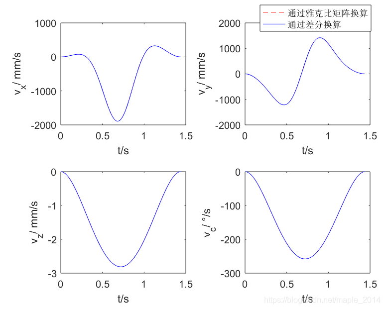
1、点到点运动
(1)在 [ − π , π ] [-\pi, \pi] [−π,π]中随机生成4个关节角度,生成点到点运动起点与终点(模拟示教过程)
(2)速度规划(详见另一篇博文:归一化5次多项式速度规划)
(3)ptp插补得到关节位置、速度、加速度
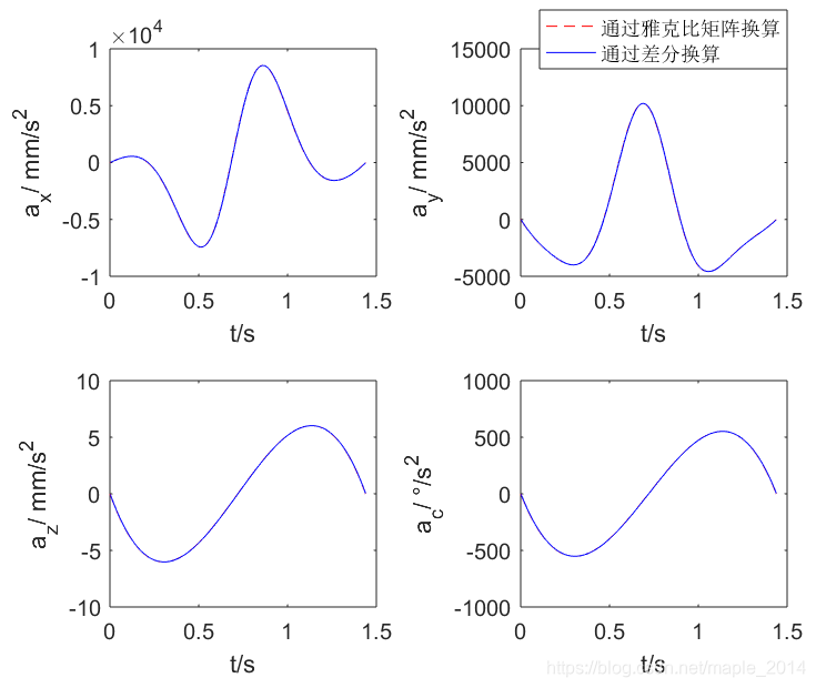
(4)运动学正解得到笛卡尔位置(x,y,z,c),并作差分运算,估计笛卡尔分轴速度、加速度
(5)利用雅克比矩阵计算笛卡尔分轴速度、加速度
(6)绘图比较(4)与(5)的差异,验证雅克比矩阵正确性
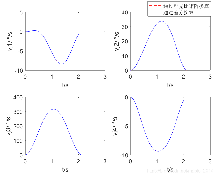
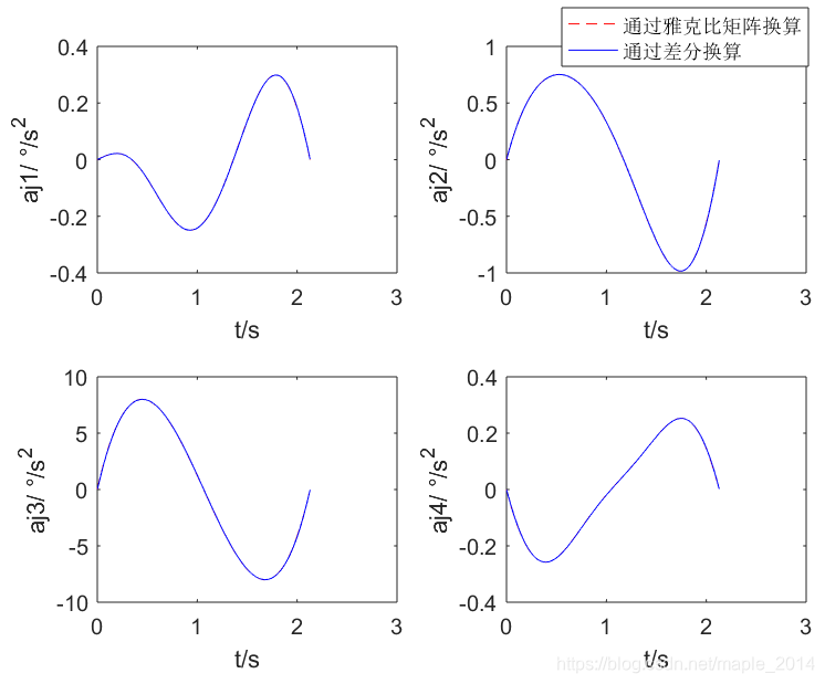
2、直线运动
(1)给定直线运动起点与终点,手系handcoor,标志位flagJ1和flagJ2(模拟示教过程)
(2)速度规划(详见另一篇博文:归一化5次多项式速度规划)
(3)直线插补得到笛卡尔位置、速度、加速度
(4)运动学逆解得到关节位置,并作差分运算,估计关节速度、加速度
(5)利用雅克比矩阵计算关节速度、加速度
(6)绘图比较(4)与(5)的差异,验证雅克比矩阵正确性
三、MATLAB代码
%{
Function: scara_forward_kinematics
Description: scara机器人运动学正解
Input: 大臂长L1(mm),小臂长L2(mm),丝杆螺距screw(mm),机器人关节位置jointPos(rad)
Output: 机器人末端位置cartesianPos(mm或rad)
Author: Marc Pony([email protected])
%}
function cartesianPos = scara_forward_kinematics(L1, L2, screw, jointPos)
theta1 = jointPos(1);
theta2 = jointPos(2);
theta3 = jointPos(3);
theta4 = jointPos(4);
x = L1 * cos(theta1) + L2 * cos(theta1 + theta2);
y = L1 * sin(theta1) + L2 * sin(theta1 + theta2);
z = theta3 * screw / (2 * pi);
c = theta1 + theta2 + theta4;
cartesianPos = [x; y; z; c];
end
%{
Function: scara_inverse_kinematics
Description: scara机器人运动学逆解
Input: 大臂长L1(mm),小臂长L2(mm),丝杆螺距screw(mm),机器人末端坐标cartesianPos(mm或rad)
       手系handcoor,标志位flagJ1与flagJ2
Output: 机器人关节位置jointPos(rad)
Author: Marc Pony([email protected])
%}
function jointPos = scara_inverse_kinematics(L1, L2, screw, cartesianPos, handcoor, flagJ1, flagJ2)
x = cartesianPos(1);
y = cartesianPos(2);
z = cartesianPos(3);
c = cartesianPos(4);
jointPos = zeros(4, 1);

calculateError = 1.0e-8;
c2 = (x^2 + y^2 - L1^2 -L2^2) / (2.0 * L1 * L2);%若(x,y)在工作空间里,则c2必在[-1,1]里,但由于计算精度,c2的绝对值可能稍微大于1
temp = 1.0 - c2^2;

if temp < 0.0
    if temp > -calculateError
        temp = 0.0;
    else
        error('区域不可到达');
    end
end
if handcoor == 0    %left handcoor
    jointPos(2) = atan2(-sqrt(temp), c2);
else                %right handcoor
    jointPos(2) = atan2(sqrt(temp), c2);
end
s2 = sin(jointPos(2));
jointPos(1) = atan2(y, x) - atan2(L2 * s2, L1 + L2 * c2);
jointPos(3) = 2.0 * pi * z / screw;

if jointPos(1) <= -pi
    jointPos(1) = jointPos(1) + 2.0*pi;
end
if jointPos(1) >= pi
    jointPos(1) = jointPos(1) - 2.0*pi;
end

if flagJ1 == 1
    if jointPos(1) >= 0.0
        jointPos(1) = jointPos(1) - 2.0*pi;
    else
        jointPos(1) = jointPos(1) + 2.0*pi;
    end
end

if flagJ2 == 1
    if jointPos(2) >= 0.0
        jointPos(2) = jointPos(2) - 2.0*pi;
    else
        jointPos(2) = jointPos(2) + 2.0*pi;
    end
end
jointPos(4) = c - jointPos(1) - jointPos(2);
end
clc;
clear;
close all;
syms L1 L2 theta1 theta2 s real
syms dtheta1 dtheta2 dtheta3 dtheta4 ddtheta1 ddtheta2 ddtheta3 ddtheta4 real
syms vx vy vz vc ax ay az ac real;

J = [-L1*sin(theta1) - L2*sin(theta1 + theta2),  -L2*sin(theta1 + theta2), 0, 0
    L1*cos(theta1) + L2*cos(theta1 + theta2),  L2*cos(theta1 + theta2), 0, 0
    0, 0, s/(2*pi), 0
    1, 1, 0, 1];
detJ = simplify(det(J))

dJ = [-L1*cos(theta1)*dtheta1 - L2*cos(theta1 + theta2)*(dtheta1 + dtheta2), -L2*cos(theta1 + theta2)*(dtheta1 + dtheta2), 0, 0
    -L1*sin(theta1)*dtheta1 - L2*sin(theta1 + theta2)*(dtheta1 + dtheta2), -L2*sin(theta1 + theta2)*(dtheta1 + dtheta2), 0, 0
    0, 0, 0, 0
    0, 0, 0, 0];

cartesianVel = simplify(J * [dtheta1; dtheta2; dtheta3; dtheta4])
cartesianAcc = simplify(dJ * [dtheta1; dtheta2; dtheta3; dtheta4] + J * [ddtheta1; ddtheta2; ddtheta3; ddtheta4])
jointVel = simplify(J \ [vx; vy; vz; vc])
jointAcc = simplify(J \ ([ax; ay; az; ac] - dJ * jointVel))

%% 输入参数
len1 = 200; %mm
len2 = 200; %mm
screw = 20; %mm
speedJ = 200; %°/s
accJ = 1200; %°/s^2
linearSpeed = 100; %mm/s
linearAcc = 800;   %mm/s^2
orientationSpeed = 200; %°/s
orientationAcc = 600;   %°/s^2
dt = 0.001; %s

%% 点到点运动, 验证雅克比矩阵正确性
%(1)在[-pi, pi]中随机生成4个关节角度,生成点到点运动起点与终点(模拟示教过程)
%(2)速度规划
%(3)ptp插补得到关节位置、速度、加速度
%(4)运动学正解得到笛卡尔位置(x,y,z,c),并作差分运算,估计笛卡尔分轴速度、加速度
%(5)利用雅克比矩阵计算笛卡尔分轴速度、加速度
%(6)绘图比较(4)与(5)的差异,验证雅克比矩阵正确性
theta = (-pi + 2.0*pi*rand(2, 4))*180.0/pi;
L = max(abs(diff(theta)));
T = max([1.875 * L / speedJ, sqrt(5.7735 * L / accJ)]);

t = (0 : dt : T)';
u = t / T;
if abs(t(end) - T) > 1.0e-8
    t = [t; T];
    u = [u; 1];
end
u = t / T;
s = 10*u.^3 - 15*u.^4 + 6*u.^5;
ds = 30*u.^2 -60*u.^3 + 30*u.^4;
dds = 60*u - 180*u.^2 + 120*u.^3;

len = L * s;
vel = (L / T) * ds;
acc = (L / T^2) * dds;
rate = diff(theta) / L;
jointPos = zeros(length(t), 4);
jointVel = zeros(length(t), 4);
jointAcc = zeros(length(t), 4);
cartesianPos = zeros(length(t), 4);
cartesianVel = zeros(length(t), 4);
cartesianAcc = zeros(length(t), 4);
for i = 1 : length(t)
    jointPos(i, :) = (theta(1, :) + len(i) * rate)*pi/180.0;
    jointVel(i, :) = (vel(i) * rate)*pi/180.0;
    jointAcc(i, :) = (acc(i) * rate)*pi/180.0;
    cartesianPos(i, :) = scara_forward_kinematics(len1, len2, screw, jointPos(i, :));
    cartesianPos(i, 4) = cartesianPos(i, 4)*180.0/pi;

    theta1 = jointPos(i, 1);
    theta2 = jointPos(i, 2);
    J = [-len1*sin(theta1) - len2*sin(theta1 + theta2),  -len2*sin(theta1 + theta2), 0, 0
        len1*cos(theta1) + len2*cos(theta1 + theta2),  len2*cos(theta1 + theta2), 0, 0
        0, 0, screw/(2*pi), 0
        1, 1, 0, 1];

    dtheta1 = jointVel(i, 1);
    dtheta2 = jointVel(i, 2);
    dtheta3 = jointVel(i, 3);
    dtheta4 = jointVel(i, 4);
    ddtheta1 = jointAcc(i, 1);
    ddtheta2 = jointAcc(i, 2);
    ddtheta3 = jointAcc(i, 3);
    ddtheta4 = jointAcc(i, 4);

    dJ = [-len1*cos(theta1)*dtheta1 - len2*cos(theta1 + theta2)*(dtheta1 + dtheta2), -len2*cos(theta1 + theta2)*(dtheta1 + dtheta2), 0, 0
        -len1*sin(theta1)*dtheta1 - len2*sin(theta1 + theta2)*(dtheta1 + dtheta2), -len2*sin(theta1 + theta2)*(dtheta1 + dtheta2), 0, 0
        0, 0, 0, 0
        0, 0, 0, 0];

    cartesianVel(i, :) = (J * [dtheta1; dtheta2; dtheta3; dtheta4])';
    cartesianAcc(i, :) = (dJ * [dtheta1; dtheta2; dtheta3; dtheta4] + J * [ddtheta1; ddtheta2; ddtheta3; ddtheta4])';
    cartesianVel(i, 4) = cartesianVel(i, 4)*180.0/pi;
    cartesianAcc(i, 4) = cartesianAcc(i, 4)*180.0/pi;
end
cartesianVel2 = diff(cartesianPos) ./ diff(t);
cartesianAcc2 = diff(cartesianVel2) ./ diff(t(2:end));

figure(1)
set(gcf, 'color','w');
subplot(2,2,1)
plot(t, cartesianVel(:, 1), '--r')
hold on
plot(t(2:end), cartesianVel2(:, 1), 'b')
xlabel('t/s');
ylabel('v_x/ mm/s');
subplot(2,2,2)
plot(t, cartesianVel(:, 2), '--r')
hold on
plot(t(2:end), cartesianVel2(:, 2), 'b')
xlabel('t/s');
ylabel('v_y/ mm/s');
legend('通过雅克比矩阵换算','通过差分换算');
subplot(2,2,3)
plot(t, cartesianVel(:, 3), '--r')
hold on
plot(t(2:end), cartesianVel2(:, 3), 'b')
xlabel('t/s');
ylabel('v_z/ mm/s');
subplot(2,2,4)
plot(t, cartesianVel(:, 4), '--r')
hold on
plot(t(2:end), cartesianVel2(:, 4), 'b')
xlabel('t/s');
ylabel('v_c/ °/s');

figure(2)
set(gcf, 'color','w');
subplot(2,2,1)
plot(t, cartesianAcc(:, 1), '--r')
hold on
plot(t(3:end), cartesianAcc2(:, 1), 'b')
xlabel('t/s');
ylabel('a_x/ mm/s^2');
subplot(2,2,2)
plot(t, cartesianAcc(:, 2), '--r')
hold on
plot(t(3:end), cartesianAcc2(:, 2), 'b')
xlabel('t/s');
ylabel('a_y/ mm/s^2');
legend('通过雅克比矩阵换算','通过差分换算');
subplot(2,2,3)
plot(t, cartesianAcc(:, 3), '--r')
hold on
plot(t(3:end), cartesianAcc2(:, 3), 'b')
xlabel('t/s');
ylabel('a_z/ mm/s^2');
subplot(2,2,4)
plot(t, cartesianAcc(:, 4), '--r')
hold on
plot(t(3:end), cartesianAcc2(:, 4), 'b')
xlabel('t/s');
ylabel('a_c/ °/s^2');

%% 直线运动, 验证雅克比矩阵正确性
%(1)给定直线运动起点与终点,手系handcoor,标志位flagJ1和flagJ2(模拟示教过程)
%(2)速度规划
%(3)直线插补得到笛卡尔位置、速度、加速度
%(4)运动学逆解得到关节位置,并作差分运算,估计关节速度、加速度
%(5)利用雅克比矩阵计算关节速度、加速度
%(6)绘图比较(4)与(5)的差异,验证雅克比矩阵正确性
handcoor = 0;
flagJ1 = 0;
flagJ2 = 0;
pos = [200 100 0 60
    250 200 20 80]; %mm °
x1 = pos(1, 1);
y1 = pos(1, 2);
z1 = pos(1, 3);
cc1 = pos(1, 4);
x2 = pos(2, 1);
y2 = pos(2, 2);
z2 = pos(2, 3);
cc2 = pos(2, 4);

L = sqrt((x2 - x1)^2 + (y2 - y1)^2 + (z2 - z1)^2);
C = abs(cc2 - cc1);
T = max([1.875 * L / linearSpeed, 1.875 * C / orientationSpeed, ...
    sqrt(5.7735 * L / linearAcc), sqrt(5.7735 * C / orientationAcc)]);

t = (0 : dt : T)';
u = t / T;
if abs(t(end) - T) > 1.0e-8
    t = [t; T];
    u = [u; 1];
end
u = t / T;
s = 10*u.^3 - 15*u.^4 + 6*u.^5;
ds = 30*u.^2 -60*u.^3 + 30*u.^4;
dds = 60*u - 180*u.^2 + 120*u.^3;

len = L * s;
vel = (L / T) * ds;
acc = (L / T^2) * dds;
cartesianPos = zeros(length(t), 4);
cartesianVel = zeros(length(t), 4);
cartesianAcc = zeros(length(t), 4);
jointPos = zeros(length(t), 4);
jointVel = zeros(length(t), 4);
jointAcc = zeros(length(t), 4);
rate = [x2 - x1, y2 - y1, z2 - z1, cc2 - cc1] / L;
for i = 1 : length(t)

    cartesianPos(i, :) = [x1, y1, z1, cc1] + len(i) * rate;
    cartesianVel(i, :) = vel(i) * rate;
    cartesianAcc(i, :) = acc(i) * rate;

    cartesianPos(i, 4) = cartesianPos(i, 4)*pi/180.0;
    jointPos(i, :) = scara_inverse_kinematics(len1, len2, screw, cartesianPos(i, :), handcoor, flagJ1, flagJ2);

    theta1 = jointPos(i, 1);
    theta2 = jointPos(i, 2);
    s1 = sin(theta1);
    s12 = sin(theta1 + theta2);
    c1 = cos(theta1);
    c12 = cos(theta1 + theta2);

    vx = cartesianVel(i, 1);
    vy = cartesianVel(i, 2);
    vz = cartesianVel(i, 3);
    vc = cartesianVel(i, 4)*pi/180.0;

    a12 = -len2*s12;
    a11 = -len1*s1 + a12;
    b1 = vx;
    a22 = len2*c12;
    a21 = len1*c1 + a22;
    b2 = vy;
    temp = a11*a22 - a12*a21;

    dtheta1 = -(a12*b2 - a22*b1)/temp;
    dtheta2 = (a11*b2 - a21*b1)/temp;
    dtheta3 = 2*pi*vz/screw;
    dtheta4 = vc - dtheta1 - dtheta2;
    jointVel(i, :) = [dtheta1, dtheta2, dtheta3, dtheta4];

    ax = cartesianAcc(i, 1);
    ay = cartesianAcc(i, 2);
    az = cartesianAcc(i, 3);
    ac = cartesianAcc(i, 4)*pi/180.0;

    d1 = ax + len1*c1*dtheta1^2 + len2*c12*(dtheta1 + dtheta2)^2;
    d2 = ay + len1*s1*dtheta1^2 + len2*s12*(dtheta1 + dtheta2)^2;
    ddtheta1 = -(a12*d2 - a22*d1)/temp;
    ddtheta2 = (a11*d2 - a21*d1)/temp;
    ddtheta3 = 2*pi*az/screw;
    ddtheta4 = ac - ddtheta1 - ddtheta2;

    jointAcc(i, :) = [ddtheta1, ddtheta2, ddtheta3, ddtheta4];
end
jointVel2 = diff(jointPos) ./ diff(t);
jointAcc2 = diff(jointVel2) ./ diff(t(2:end));

figure(3)
set(gcf, 'color','w');
subplot(2,2,1)
plot(t, jointVel(:, 1)*180.0/pi, '--r')
hold on
plot(t(2:end), jointVel2(:, 1)*180.0/pi, 'b')
xlabel('t/s');
ylabel('vj1/ °/s');
subplot(2,2,2)
plot(t, jointVel(:, 2)*180.0/pi, '--r')
hold on
plot(t(2:end), jointVel2(:, 2)*180.0/pi, 'b')
xlabel('t/s');
ylabel('vj2/ °/s');
legend('通过雅克比矩阵换算','通过差分换算');
subplot(2,2,3)
plot(t, jointVel(:, 3)*180.0/pi, '--r')
hold on
plot(t(2:end), jointVel2(:, 3)*180.0/pi, 'b')
xlabel('t/s');
ylabel('vj3/ °/s');
subplot(2,2,4)
plot(t, jointVel(:, 4)*180.0/pi, '--r')
hold on
plot(t(2:end), jointVel2(:, 4)*180.0/pi, 'b')
xlabel('t/s');
ylabel('vj4/ °/s');

figure(4)
set(gcf, 'color','w');
subplot(2,2,1)
plot(t, jointAcc(:, 1), '--r')
hold on
plot(t(3:end), jointAcc2(:, 1), 'b')
xlabel('t/s');
ylabel('aj1/ °/s^2');
subplot(2,2,2)
plot(t, jointAcc(:, 2), '--r')
hold on
plot(t(3:end), jointAcc2(:, 2), 'b')
xlabel('t/s');
ylabel('aj2/ °/s^2');
legend('通过雅克比矩阵换算','通过差分换算');
subplot(2,2,3)
plot(t, jointAcc(:, 3), '--r')
hold on
plot(t(3:end), jointAcc2(:, 3), 'b')
xlabel('t/s');
ylabel('aj3/ °/s^2');
subplot(2,2,4)
plot(t, jointAcc(:, 4), '--r')
hold on
plot(t(3:end), jointAcc2(:, 4), 'b')
xlabel('t/s');
ylabel('aj4/ °/s^2');