原理
Fourier Transform is used to analyze the frequency characteristics of various filters. For images, 2D Discrete Fourier Transform (DFT) is used to find the frequency domain. A fast algorithm called Fast Fourier Transform (FFT) is used for calculation of DFT. Details about these can be found in any image processing or signal processing textbooks. Please see Additional Resources_ section.
For a sinusoidal signal, x(t)=Asin(2πft), we can say f is the frequency of signal, and if its frequency domain is taken, we can see a spike at f. If signal is sampled to form a discrete signal, we get the same frequency domain, but is periodic in the range [−π,π] or [0,2π] (or [0,N] for N-point DFT). You can consider an image as a signal which is sampled in two directions. So taking fourier transform in both X and Y directions gives you the frequency representation of image.
More intuitively, for the sinusoidal signal, if the amplitude varies so fast in short time, you can say it is a high frequency signal. If it varies slowly, it is a low frequency signal. You can extend the same idea to images. Where does the amplitude varies drastically in images ? At the edge points, or noises. So we can say, edges and noises are high frequency contents in an image. If there is no much changes in amplitude, it is a low frequency component. ( Some links are added to Additional Resources_ which explains frequency transform intuitively with examples).
Now we will see how to find the Fourier Transform.
把图像想象成沿着两个方向采集的信号。所以对图像同时进行 X 方向和 Y 方向的傅里叶变换,我们就会得到这幅图像的频域表示(频谱图)。更直观一点,对于一个正弦信号,如果它的幅值变化非常快,我们可以说它是高频信号,如果变化非常慢,我们称之为低频信号。把这种想法应用到图像中,图像哪里的幅度变化非常大呢?边界点或者噪声。所以我们说边界和噪声是图像中的高频分量。
Numpy 中的傅里叶变换
First we will see how to find Fourier Transform using Numpy. Numpy has an FFT package to do this. np.fft.fft2() provides us the frequency transform which will be a complex array. Its first argument is the input image, which is grayscale. Second argument is optional which decides the size of output array. If it is greater than size of input image, input image is padded with zeros before calculation of FFT. If it is less than input image, input image will be cropped. If no arguments passed, Output array size will be same as input.
Now once you got the result, zero frequency component (DC component) will be at top left corner. If you want to bring it to center, you need to shift the result by N2 in both the directions. This is simply done by the function, np.fft.fftshift(). (It is more easier to analyze). Once you found the frequency transform, you can find the magnitude spectrum.
Numpy 中的 FFT 包 可以帮助我们实现快速傅里叶变换。函数 np.fft.fft2() 可以对信号进行频率转换,输出结果是一个复杂的组。本函数的第一个参数是输入图像,要求是灰度格式。第二个参数是可选的, 决定输出数组的大小。输出数组的大小和输入图像大小一样。如果输出结果比输入图像大,输入图像就需要在进行 FFT 前补0。如果输出结果比输入图像小的话,输入图像就会被切割。
现在我们得到了结果,频率为 0 的部分(直流分量)在输出图像的左上角。如果想让它(直流分量)在输出图像的中心,我们还需要将结果沿两个方向平移 N/2 。函数 np.fft.fftshift() 可以帮助我们实现这一步。(这样更容易分析)。进行完频率变换之后,我们就可以构建振幅谱了。
代码
import cv2 as cv
import numpy as np
from matplotlib import pyplot as plt
img = cv.imread('6.jpg',0)
f = np.fft.fft2(img)
fshift = np.fft.fftshift(f)
magnitude_spectrum = 20*np.log(np.abs(fshift))
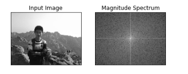
plt.subplot(121),plt.imshow(img, cmap = 'gray')
plt.title('Input Image'), plt.xticks([]), plt.yticks([])
plt.subplot(122),plt.imshow(magnitude_spectrum, cmap = 'gray')
plt.title('Magnitude Spectrum'), plt.xticks([]), plt.yticks([])
plt.show()