说说优秀的目标识别yolov3算法
前言
yolo系列一直是我喜欢的算法,虽然yolov4出来了很久了,但是yolov3还是具有很大的研究空间。今天我们来解析下yolov3.(虽然我以前写过,但是我最近对这个算法有了新的理解)

论文地址
https://pjreddie.com/media/files/papers/YOLOv3.pdf
github地址
https://github.com/yanjingke/yolo3
预备知识
ps:花10分钟理解
Yolov3边框预测
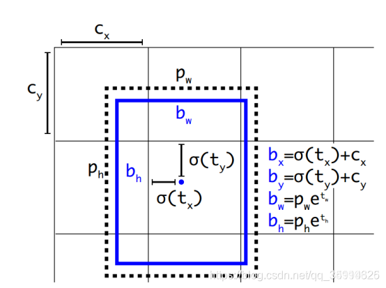
论文中边框预测公式如下:

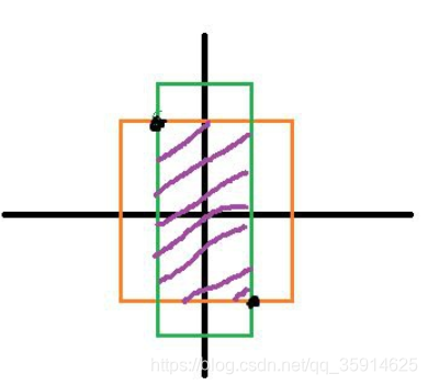
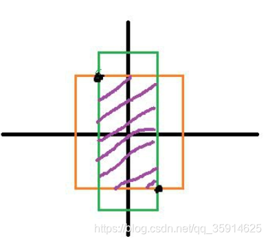
其中,Cx,Cy是feature map中真实框的左上角坐标,在yolov3中每个grid cell在feature map中的宽和高均为1。在下面情况中bbox边界框的中心属于第二行第二列的真实框,它的左上角坐标为(1,1),故Cx=1,Cy=1.公式中的Pw、Ph是预设的anchor box映射到feature map中的宽和高。 最终得到的边框坐标值是bx,by,bw,bh即边界框bbox相对于feature map的位置和大小,是我们需要的预测输出坐标。但我们网络实际上的学习目标是tx,ty,tw,th这4个offsets,其中tx,ty是预测的坐标偏移值,tw,th是尺度缩放,有了这4个offsets,自然可以根据之前的公式去求得真正需要的bx,by,bw,bh4个坐标。
这里解释一下anchor box,YOLO3为每种FPN预测特征图(13x13,26x26,52x52)设定3种anchor box,总共聚类(这里大家如果想聚类可以自己使用我代码的kmeans_for_anchors.py)出9种尺寸的anchor box。在COCO数据集这9个anchor box是:(10x13),(16x30),(33x23),(30x61),(62x45),(59x119),(116x90),(156x198),(373x326)。分配上,在最小的13x13特征图上由于其感受野最大故应用最大的anchor box (116x90),(156x198),(373x326)。适合检测较大的目标。中等的26x26特征图上由于其具有中等感受野故应用中等的anchor box (30x61),(62x45),(59x119),适合检测中等大小的目标。较大的52x52特征图上由于其具有较小的感受野故应用最小的anchor box(10x13),(16x30),(33x23),适合检测较小的目标。同Faster-Rcnn一样,特征图的每个像素(即每个grid)都会有对应的三个anchor box,如13*13特征图的每个grid都有三个anchor box (116x90),(156x198),(373x326)(这几个坐标需除以32缩放尺寸)
代码:
def yolo_head(feats, anchors, num_classes, input_shape, calc_loss=False):
    num_anchors = len(anchors)
    # [1, 1, 1, num_anchors, 2]-.(1,1,1,3,2)
    anchors_tensor = K.reshape(K.constant(anchors), [1, 1, 1, num_anchors, 2])

    # 获得x,y的网格
    # (13, 13, 1, 2)
    grid_shape = K.shape(feats)[1:3] # # height, width (?,13,13,255)  -> (13,13)
    #13,1,1,1-> shape=(13, 13, 1, 1)
    grid_y = K.tile(K.reshape(K.arange(0, stop=grid_shape[0]), [-1, 1, 1, 1]),
        [1, grid_shape[1], 1, 1])
    #1,13,1,1->shape=(13,13,1,1)
    grid_x = K.tile(K.reshape(K.arange(0, stop=grid_shape[1]), [1, -1, 1, 1]),
        [grid_shape[0], 1, 1, 1])
    #13,13,1,2
    grid = K.concatenate([grid_x, grid_y])
    grid = K.cast(grid, K.dtype(feats))

    # (batch_size,13,13,3,85)最后一个维度中的85包含了4+1+80,分别代表x_offset、y_offset、h和w、置信度、分类结果。
    feats = K.reshape(feats, [-1, grid_shape[0], grid_shape[1], num_anchors, num_classes + 5])

    # 将预测值调成真实值
    # box_xy对应框的中心点
    # box_wh对应框的宽和高
    #所以a[::-1]相当于 a[-1:-len(a)-1:-1],也就是从最后一个元素到第一个元素复制一遍,即倒序。
    box_xy = (K.sigmoid(feats[..., :2]) + grid) / K.cast(grid_shape[::-1], K.dtype(feats))
    box_wh = K.exp(feats[..., 2:4]) * anchors_tensor / K.cast(input_shape[::-1], K.dtype(feats))
    box_confidence = K.sigmoid(feats[..., 4:5])
    box_class_probs = K.sigmoid(feats[..., 5:])

    # 在计算loss的时候返回如下参数
    if calc_loss == True:
        return grid, feats, box_xy, box_wh
    return box_xy, box_wh, box_confidence, box_class_probs
Yolov3边框解码
解码的操作是为了在训练时方便与预测值作为对比,用来计算loss。在faster RCNN中解码其公式如下图,Px,Py在是预设的anchor box在feature map上的中心角坐标。 Pw、Ph是预设的anchor box的在feature map上的宽和高。至于Gx、Gy、Gw、Gh自然就是ground truth在这个feature map的4个坐标了。用x,y坐标减去anchor box的x,y坐标得到偏移量好理解,**为何要除以feature map上anchor box的宽和高呢?**我认为可能是为了把绝对尺度变为相对尺度,毕竟作为偏移量,不能太大了对吧。而且不同尺度的anchor box如果都用Gx-Px来衡量显然不对,有的anchor box大有的却很小,都用Gx-Px会导致不同尺度的anchor box权重相同,而大的anchor box肯定更能容忍大点的偏移量,小的anchor box对小偏移都很敏感,故除以宽和高可以权衡不同尺度下的预测坐标偏移量。
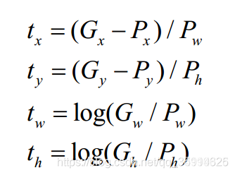
但是在yolov3中与faster-rcnn系列文章用到的公式在前两行是不同的,yolov3里Px和Py就换为了feature map上的grid cell左上角坐标Cx,Cy了,即在yolov3里是Gx,Gy减去grid cell左上角坐标Cx,Cy。x,y坐标并没有针对anchon box求偏移量,所以并不需要除以Pw,Ph。
也就是说是tx = Gx - Cx
ty = Gy - Cy
这样就可以直接求bbox中心距离真实框左上角的坐标的偏移量。
对于某个ground truth框,究竟是哪个anchor负责匹配它呢?和YOLOv1一样,对于训练图片中的ground truth,若其中心点落在某个cell内,那么该cell内的3个anchor box负责预测它,具体是哪个anchor box预测它,需要在训练中确定,即由那个与ground truth的IOU最大的anchor box预测它,而剩余的2个anchor box不与该ground truth匹配。YOLOv3需要假定每个cell至多含有一个grounth truth,而在实际上基本不会出现多于1个的情况。与ground truth匹配的anchor box计算坐标误差、置信度误差(此时target为1)以及分类误差,而其它的anchor box只计算置信度误差(此时target为0)。有了平移(tx,ty)和尺度缩放(tw,th)才能让anchor box经过微调与grand truth重合。利用边框回归最简单的想法就是通过平移加尺度缩放进行微调嘛。
那么训练时用的groundtruth的4个坐标去做差值和比值得到tx,ty,tw,th,测试时就用预测的bbox就好了,公式修改就简单了,把Gx和Gy改为预测的x,y,Gw、Gh改为预测的w,h即可。
网络可以不断学习tx,ty,tw,th偏移量和尺度缩放,预测时使用这4个offsets求得bx,by,bw,bh即可,那么问题是:tx,ty为何要sigmoid一下啊?
前面讲到了在yolov3中没有让Gx - Cx后除以Pw得到tx,而是直接Gx - Cx得到tx,这样会有问题是导致tx比较大且很可能>1.(因为没有除以Pw归一化尺度。一旦tx,ty算出来大于1就会落入必须其他真实框中,而不能出现在它旁边网格中,引起矛盾,因而必须归一化。

代码讲解
预测部分
主干特征提取darkNet53
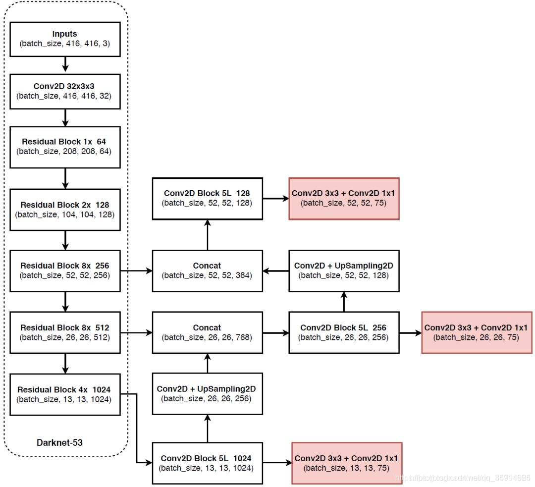
它采用了一个新的网络来提取特征,它融合了YOLOv2、Darknet-19以及其他新型残差网络,由连续的3×3和1×1卷积层组合而成,当然,其中也添加了一些shortcut connection,整体体量也更大。因为一共有53个卷积层,所以叫做称它为Darknet-53。
Darknet-53
1.采用Inverted residual在3x3网络结构前利用1x1卷积降维,在3x3网络结构后,利用1x1卷积升维,相比直接使用3x3网络卷积效果更好,参数更少,先进行压缩,再进行扩张。
2.采用残差网络,后面的特征层的内容会有一部分由其前面的某一层线性贡献。
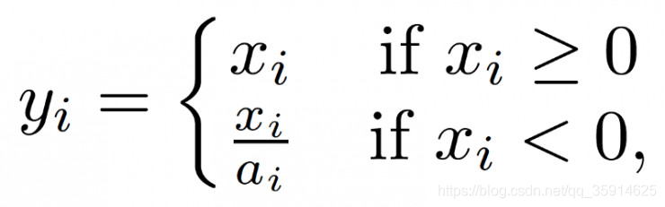
3.采用Leaky ReLUs, ReLU是将所有的负值都设为零,相反,Leaky ReLU是给所有负值赋予一个非零斜率。Leaky ReLU激活函数是在声学模型(2013)中首次提出的。以数学的方式我们可以表示为:

from functools import wraps
from keras.layers import Conv2D, Add, ZeroPadding2D, UpSampling2D, Concatenate, MaxPooling2D
from keras.layers.advanced_activations import LeakyReLU
from keras.layers.normalization import BatchNormalization
from keras.regularizers import l2
from utils.utils import compose


#--------------------------------------------------#
#   单次卷积
#--------------------------------------------------#
@wraps(Conv2D)
def DarknetConv2D(*args, **kwargs):
    darknet_conv_kwargs = {'kernel_regularizer': l2(5e-4)}
    darknet_conv_kwargs['padding'] = 'valid' if kwargs.get('strides')==(2,2) else 'same'
    darknet_conv_kwargs.update(kwargs)
    return Conv2D(*args, **darknet_conv_kwargs)

#---------------------------------------------------#
#   卷积块
#   DarknetConv2D + BatchNormalization + LeakyReLU
#---------------------------------------------------#
def DarknetConv2D_BN_Leaky(*args, **kwargs):
    no_bias_kwargs = {'use_bias': False}
    no_bias_kwargs.update(kwargs)
    return compose(
        DarknetConv2D(*args, **no_bias_kwargs),
        BatchNormalization(),
        LeakyReLU(alpha=0.1))

#---------------------------------------------------#
#   卷积块
#   DarknetConv2D + BatchNormalization + LeakyReLU
#---------------------------------------------------#
def resblock_body(x, num_filters, num_blocks):
    x = ZeroPadding2D(((1,0),(1,0)))(x)
    x = DarknetConv2D_BN_Leaky(num_filters, (3,3), strides=(2,2))(x)
    for i in range(num_blocks):
        y = DarknetConv2D_BN_Leaky(num_filters//2, (1,1))(x)
        y = DarknetConv2D_BN_Leaky(num_filters, (3,3))(y)
        x = Add()([x,y])
    return x

#---------------------------------------------------#
#   darknet53 的主体部分
#---------------------------------------------------#
def darknet_body(x):
    x = DarknetConv2D_BN_Leaky(32, (3,3))(x)
    x = resblock_body(x, 64, 1)
    x = resblock_body(x, 128, 2)
    x = resblock_body(x, 256, 8)
    feat1 = x
    x = resblock_body(x, 512, 8)
    feat2 = x
    x = resblock_body(x, 1024, 4)
    feat3 = x
    return feat1,feat2,feat3
特征金字塔构建,获得预测结果
通过前面的特征提取我们获得五个特征层,分别是feat1、feat2、feat3,7。他们的大小分别是(52x52x256)(26x26x512)(13x13x1024)
三个特征层进行5次卷积处理,处理完后一部分用于输出该特征层对应的预测结果,一部分用于进行反卷积UmSampling2d后与其它特征层进行结合。输出层的shape分别为(13,13,255),(26,26,255),(52,52,255),最后一个维度为255是因为该图是基于coco数据集的,85包含了4+1+80,分别代表x_offset、y_offset、h和w、置信度(是否有对象的概率)、分类结果。coco数据集种类为80种,yolo3只有针对每一个特征层存在3个先验框,所以最后维度为3x(4+1+80)。
#--------------------------------------------------#
#   单次卷积
#--------------------------------------------------#
@wraps(Conv2D)
def DarknetConv2D(*args, **kwargs):
    darknet_conv_kwargs = {'kernel_regularizer': l2(5e-4)}
    darknet_conv_kwargs['padding'] = 'valid' if kwargs.get('strides')==(2,2) else 'same'
    darknet_conv_kwargs.update(kwargs)
    return Conv2D(*args, **darknet_conv_kwargs)

#---------------------------------------------------#
#   卷积块
#   DarknetConv2D + BatchNormalization + LeakyReLU
#---------------------------------------------------#
def DarknetConv2D_BN_Leaky(*args, **kwargs):
    no_bias_kwargs = {'use_bias': False}
    no_bias_kwargs.update(kwargs)
    return compose(
        DarknetConv2D(*args, **no_bias_kwargs),
        BatchNormalization(),
        LeakyReLU(alpha=0.1))

#---------------------------------------------------#
#   特征层->最后的输出
#---------------------------------------------------#
def make_last_layers(x, num_filters, out_filters):
    # 五次卷积
    x = DarknetConv2D_BN_Leaky(num_filters, (1,1))(x)
    x = DarknetConv2D_BN_Leaky(num_filters*2, (3,3))(x)
    x = DarknetConv2D_BN_Leaky(num_filters, (1,1))(x)
    x = DarknetConv2D_BN_Leaky(num_filters*2, (3,3))(x)
    x = DarknetConv2D_BN_Leaky(num_filters, (1,1))(x)

    # 将最后的通道数调整为outfilter
    y = DarknetConv2D_BN_Leaky(num_filters*2, (3,3))(x)
    y = DarknetConv2D(out_filters, (1,1))(y)

    return x, y

#---------------------------------------------------#
#   特征层->最后的输出
#---------------------------------------------------#
def yolo_body(inputs, num_anchors, num_classes):
    # 生成darknet53的主干模型
    feat1,feat2,feat3 = darknet_body(inputs)
    darknet = Model(inputs, feat3)

    # 第一个特征层
    # y1=(batch_size,13,13,3,85)
    x, y1 = make_last_layers(darknet.output, 512, num_anchors*(num_classes+5))

    x = compose(
            DarknetConv2D_BN_Leaky(256, (1,1)),
            UpSampling2D(2))(x)
    x = Concatenate()([x,feat2])
    # 第二个特征层
    # y2=(batch_size,26,26,3,85)
    x, y2 = make_last_layers(x, 256, num_anchors*(num_classes+5))

    x = compose(
            DarknetConv2D_BN_Leaky(128, (1,1)),
            UpSampling2D(2))(x)
    x = Concatenate()([x,feat1])
    # 第三个特征层
    # y3=(batch_size,52,52,3,85)
    x, y3 = make_last_layers(x, 128, num_anchors*(num_classes+5))

    return Model(inputs, [y1,y2,y3])
预测结果的解码(可以看预备知识)
预测框的解码部分,我们通过主干网络和特征金字塔获得了
num_priors x 4的卷积 用于预测 该特征层上 每一个网格点上 每一个先验框的变化情况。
num_priors x (num_classes+1)的卷积 用于预测 该特征层上 每一个网格点上 每一个预测框对应的种类和是否包含物体。
利用预设好的 预先设定好的3个anchor框进行调整。
先验框虽然可以代表一定的框的位置信息与框的大小信息,但是其是有限的,无法表示任意情况,因此还需要调整,num_priors x (80+5)的卷积的结果对先验框进行调整。85包含了4+1+80,分别代表x_offset、y_offset、h和w、置信度、分类结果。yolov3将每个网格点加上它对应的x_offset和y_offset,加完后的结果就是预测框的中心,然后再利用 先验框和h、w结合 计算出预测框的长和宽。这样就能得到整个预测框的位置了。
#---------------------------------------------------#
#   将预测值的每个特征层调成真实值
#---------------------------------------------------#
def yolo_head(feats, anchors, num_classes, input_shape, calc_loss=False):
    num_anchors = len(anchors)
    # [1, 1, 1, num_anchors, 2]
    anchors_tensor = K.reshape(K.constant(anchors), [1, 1, 1, num_anchors, 2])

    # 获得x,y的网格
    # (13, 13, 1, 2)
    grid_shape = K.shape(feats)[1:3] # height, width
    grid_y = K.tile(K.reshape(K.arange(0, stop=grid_shape[0]), [-1, 1, 1, 1]),
        [1, grid_shape[1], 1, 1])
    grid_x = K.tile(K.reshape(K.arange(0, stop=grid_shape[1]), [1, -1, 1, 1]),
        [grid_shape[0], 1, 1, 1])
    grid = K.concatenate([grid_x, grid_y])
    grid = K.cast(grid, K.dtype(feats))

    # (batch_size,13,13,3,85)
    feats = K.reshape(feats, [-1, grid_shape[0], grid_shape[1], num_anchors, num_classes + 5])

    # 将预测值调成真实值
    # box_xy对应框的中心点
    # box_wh对应框的宽和高
    box_xy = (K.sigmoid(feats[..., :2]) + grid) / K.cast(grid_shape[::-1], K.dtype(feats))
    box_wh = K.exp(feats[..., 2:4]) * anchors_tensor / K.cast(input_shape[::-1], K.dtype(feats))
    box_confidence = K.sigmoid(feats[..., 4:5])
    box_class_probs = K.sigmoid(feats[..., 5:])

    # 在计算loss的时候返回如下参数
    if calc_loss == True:
        return grid, feats, box_xy, box_wh
    return box_xy, box_wh, box_confidence, box_class_probs

#---------------------------------------------------#
#   对box进行调整,使其符合真实图片的样子
#---------------------------------------------------#
def yolo_correct_boxes(box_xy, box_wh, input_shape, image_shape):
    box_yx = box_xy[..., ::-1]
    box_hw = box_wh[..., ::-1]

    input_shape = K.cast(input_shape, K.dtype(box_yx))
    image_shape = K.cast(image_shape, K.dtype(box_yx))

    new_shape = K.round(image_shape * K.min(input_shape/image_shape))
    offset = (input_shape-new_shape)/2./input_shape
    scale = input_shape/new_shape

    box_yx = (box_yx - offset) * scale
    box_hw *= scale

    box_mins = box_yx - (box_hw / 2.)
    box_maxes = box_yx + (box_hw / 2.)
    boxes =  K.concatenate([
        box_mins[..., 0:1],  # y_min
        box_mins[..., 1:2],  # x_min
        box_maxes[..., 0:1],  # y_max
        box_maxes[..., 1:2]  # x_max
    ])

    boxes *= K.concatenate([image_shape, image_shape])
    return boxes

#---------------------------------------------------#
#   获取每个box和它的得分
#---------------------------------------------------#
def yolo_boxes_and_scores(feats, anchors, num_classes, input_shape, image_shape):
    # 将预测值调成真实值
    # box_xy对应框的中心点
    # box_wh对应框的宽和高
    # -1,13,13,3,2; -1,13,13,3,2; -1,13,13,3,1; -1,13,13,3,80
    box_xy, box_wh, box_confidence, box_class_probs = yolo_head(feats, anchors, num_classes, input_shape)
    # 将box_xy、和box_wh调节成y_min,y_max,xmin,xmax
    boxes = yolo_correct_boxes(box_xy, box_wh, input_shape, image_shape)
当然得到最终的获得真实框的调整结果后,取出取出每一类得分大于confidence_threshold的框和得分。利用框的位置和得分进行非极大抑制,得到最终结果。
#---------------------------------------------------#
#   图片预测
#---------------------------------------------------#
def yolo_eval(yolo_outputs,
              anchors,
              num_classes,
              image_shape,
              max_boxes=20,
              score_threshold=.6,
              iou_threshold=.5):
    # 获得特征层的数量
    num_layers = len(yolo_outputs)
    # 特征层1对应的anchor是678
    # 特征层2对应的anchor是345
    # 特征层3对应的anchor是012
    anchor_mask = [[6,7,8], [3,4,5], [0,1,2]]

    input_shape = K.shape(yolo_outputs[0])[1:3] * 32
    boxes = []
    box_scores = []
    # 对每个特征层进行处理
    for l in range(num_layers):
        _boxes, _box_scores = yolo_boxes_and_scores(yolo_outputs[l], anchors[anchor_mask[l]], num_classes, input_shape, image_shape)
        boxes.append(_boxes)
        box_scores.append(_box_scores)
    # 将每个特征层的结果进行堆叠
    boxes = K.concatenate(boxes, axis=0)
    box_scores = K.concatenate(box_scores, axis=0)

    mask = box_scores >= score_threshold
    max_boxes_tensor = K.constant(max_boxes, dtype='int32')
    boxes_ = []
    scores_ = []
    classes_ = []
    for c in range(num_classes):
        # 取出所有box_scores >= score_threshold的框,和成绩
        class_boxes = tf.boolean_mask(boxes, mask[:, c])
        class_box_scores = tf.boolean_mask(box_scores[:, c], mask[:, c])

        # 非极大抑制,去掉box重合程度高的那一些
        nms_index = tf.image.non_max_suppression(
            class_boxes, class_box_scores, max_boxes_tensor, iou_threshold=iou_threshold)

        # 获取非极大抑制后的结果
        # 下列三个分别是
        # 框的位置,得分与种类
        class_boxes = K.gather(class_boxes, nms_index)
        class_box_scores = K.gather(class_box_scores, nms_index)
        classes = K.ones_like(class_box_scores, 'int32') * c
        boxes_.append(class_boxes)
        scores_.append(class_box_scores)
        classes_.append(classes)
    boxes_ = K.concatenate(boxes_, axis=0)
    scores_ = K.concatenate(scores_, axis=0)
    classes_ = K.concatenate(classes_, axis=0)

    return boxes_, scores_, classes_
训练部分
真实框的编码
实际上用于训练的的数据是经过input_shape归一化后的,所以要对标注的数据进行归一化。标注的是左上角和右下角的坐标,所在归一化前需要把标注变成标注框的中心和长宽的形式。同时,对于一个标注边框而言,作者说:“our system only assigns one bounding box prior for each ground truth object.”也就是说,对于一个标注,只能有一个最佳的anchor与之匹配(其实还没捋顺)这个最佳通过IoU来判断。
首先判断类别正常。然后按照feature map的grid的大小将anchor划分。第一层对应较大的anchor,因为该feature map 对应的感受野大。
    assert (true_boxes[..., 4]<num_classes).all(), 'class id must be less than num_classes'
    # 一共有三个特征层数
    num_layers = len(anchors)//3
    # 先验框
    # 678为116,90,  156,198,  373,326
    # 345为30,61,  62,45,  59,119
    # 012为10,13,  16,30,  33,23,
    anchor_mask = [[6,7,8], [3,4,5], [0,1,2]] if num_layers==3 else [[3,4,5], [1,2,3]]
先将标注边框的两点坐标的形式,转化为训练的中心加边长的形式。并进行归一化。这里应该是boxes_wh 的高宽与input_shape的高宽顺序不一样。
    true_boxes = np.array(true_boxes, dtype='float32')
    input_shape = np.array(input_shape, dtype='int32') # 416,416
    # 读出xy轴,读出长宽
    # 中心点(m,n,2)
    boxes_xy = (true_boxes[..., 0:2] + true_boxes[..., 2:4]) // 2
    boxes_wh = true_boxes[..., 2:4] - true_boxes[..., 0:2]
    # 计算比例
    true_boxes[..., 0:2] = boxes_xy/input_shape[:]
    true_boxes[..., 2:4] = boxes_wh/input_shape[:]
y_ture的初始化。可知y_ture有三个子项,分别对应着13x13,26x26,52x52的三个输出。也就是三个检测器的输入。每个子项的形式,去第一个,(13,13,3,5+num_classes),3代表每一个13x13的feature map的一个元素(?不止有一个数,是一个矩阵)对应着3个anchor。5代表这位置大小和置信度(1)。num_classes是一个one_hot编码。
  # m张图
    m = true_boxes.shape[0]
    # 得到网格的shape为13,13;26,26;52,52

    # for l in range(num_layers):
    #     #     # print({0: 32, 1: 16, 2: 8}[l])
    #字典
    grid_shapes = [input_shape//{0:32, 1:16, 2:8}[l] for l in range(num_layers)]
    # y_true的格式为(m,13,13,3,85)(m,26,26,3,85)(m,52,52,3,85)
    y_true = [np.zeros((m,grid_shapes[l][0],grid_shapes[l][1],len(anchor_mask[l]),5+num_classes),
        dtype='float32') for l in range(num_layers)]
第一增加维度是为更好的计算。而anchor/2和取反则是为了计算IoU。可以看作把anchor的中心移到坐标原点,boxes也进行相似的处理。valid_mask主要是有一张图片不一定有20个物体,要把有效边框找出来。(true_boxes: array, shape=(m, T, 5))
  # [1,9,2]
    anchors = np.expand_dims(anchors, 0)
    #而anchor/2和取反则是为了计算IoU。可以看作把anchor的中心移到坐标原点
    anchor_maxes = anchors / 2.
    anchor_mins = -anchor_maxes
        # 长宽要大于0才有效
    valid_mask = boxes_wh[..., 0]>0
遍历整个batch,依次对每一张的图片进行处理( for b in range(m))。
    for b in range(m):
        # 对每一张图进行处理
        wh = boxes_wh[b, valid_mask[b]]
        if len(wh)==0: continue
        # [n,1,2]
        wh = np.expand_dims(wh, -2)
        box_maxes = wh / 2.
        box_mins = -box_maxes

        # 计算真实框和哪个先验框最契合、对于有效的边框,采用与anchor相似的处理方法。
        #4,1,2
        #1,9,2
        intersect_mins = np.maximum(box_mins, anchor_mins)
        intersect_maxes = np.minimum(box_maxes, anchor_maxes)
        intersect_wh = np.maximum(intersect_maxes - intersect_mins, 0.)
        intersect_area = intersect_wh[..., 0] * intersect_wh[..., 1]
        box_area = wh[..., 0] * wh[..., 1]
        anchor_area = anchors[..., 0] * anchors[..., 1]
        iou = intersect_area / (box_area + anchor_area - intersect_area)
        # 维度是(n) 感谢 消尽不死鸟 的提醒
        best_anchor = np.argmax(iou, axis=-1)

        for t, n in enumerate(best_anchor):
            for l in range(num_layers):
                if n in anchor_mask[l]:
                    # floor用于向下取整
                    i = np.floor(true_boxes[b, t, 0] * grid_shapes[l][1]).astype('int32')  # 中心点x在grid中对应的位置
                    j = np.floor(true_boxes[b, t, 1] * grid_shapes[l][0]).astype('int32')
                    k = anchor_mask[l].index(n)  # 返回真实框对应最契合的先验框
                    c = true_boxes[b, t, 4].astype('int32')  # 该框所对应的类别(class)
                    # 将真实框的信息放进y_true与之对应的特征层的相对应中心点中
                    y_true[l][b, j, i, k, 0:4] = true_boxes[b, t, 0:4]
                    y_true[l][b, j, i, k, 4] = 1  # 置信度,表示有需要检测的物体
                    y_true[l][b, j, i, k, 5 + c] = 1  # 类别,类似于one_hot编码
对于有效的边框,采用与anchor相似的处理方法。
   # 对每一张图进行处理
        wh = boxes_wh[b, valid_mask[b]]
        if len(wh)==0: continue
        # [n,1,2]
        wh = np.expand_dims(wh, -2)
        box_maxes = wh / 2.
        box_mins = -box_maxes
计算重合度最好的iou
        # 计算真实框和哪个先验框最契合、对于有效的边框,采用与anchor相似的处理方法。
        #4,1,2
        #1,9,2
        intersect_mins = np.maximum(box_mins, anchor_mins)
        intersect_maxes = np.minimum(box_maxes, anchor_maxes)
        intersect_wh = np.maximum(intersect_maxes - intersect_mins, 0.)
        intersect_area = intersect_wh[..., 0] * intersect_wh[..., 1]
        box_area = wh[..., 0] * wh[..., 1]
        anchor_area = anchors[..., 0] * anchors[..., 1]
        iou = intersect_area / (box_area + anchor_area - intersect_area)
        # 维度是(n) 感谢 消尽不死鸟 的提醒
        best_anchor = np.argmax(iou, axis=-1)
寻找最合适的anchor,也就是一个ground truth box只与一个最佳的anchor box对应。
 for t, n in enumerate(best_anchor):
            for l in range(num_layers):
                if n in anchor_mask[l]:
                    # floor用于向下取整
                    i = np.floor(true_boxes[b, t, 0] * grid_shapes[l][1]).astype('int32')  # 中心点x在grid中对应的位置
                    j = np.floor(true_boxes[b, t, 1] * grid_shapes[l][0]).astype('int32')
                    k = anchor_mask[l].index(n)  # 返回真实框对应最契合的先验框
                    c = true_boxes[b, t, 4].astype('int32')  # 该框所对应的类别(class)
                    # 将真实框的信息放进y_true与之对应的特征层的相对应中心点中
                    y_true[l][b, j, i, k, 0:4] = true_boxes[b, t, 0:4]
                    y_true[l][b, j, i, k, 4] = 1  # 置信度,表示有需要检测的物体
                    y_true[l][b, j, i, k, 5 + c] = 1  # 类别,类似于one_hot编码
loss值计算
正负样本是按照以下规则决定的:
如果一个预测框与所有的Ground Truth的最大IoU<ignore_thresh时,那这个预测框就是负样本。
如果Ground Truth的中心点落在一个区域中,该区域就负责检测该物体。将与该物体有最大IoU的预测框作为正样本(注意这里没有用到ignore thresh,即使该最大IoU<ignore thresh也不会影响该预测框为正样本)
loss函数分四部分:
(1)计算xy(物体中心坐标)的损失
object_mask就是置信度
box_loss_scale可以理解为2-wxh
raw_true_xy就是真实的xy坐标点了
raw_pred[…, :2]是xy预测坐标点
所以第一个式子想对还挺直观,简化为: 
bool是置信度
其中bce是xy值的二值交叉熵损失,这个值越小整个损失值越小
boolx(2-areaPred)的值越小,则需要在确保置信度(bool)的情况下,areaPred需要越大。因此,这部分损失主要优化xy的预测值(bce)和置信度(bool)以及wh回归值(areaPred)
(2)计算wh(anchor长宽回归值)的损失
跟(1)式 的差距就在最后一项,所以我们直接简化之:whloss=boolx(2-areaPred) x(whtrue-whpred)^2,在确保置信度(bool)的情况下,areaPred需要越大,wh需要尽可能靠近真实值wh,这部分主要优化置信度(bool)wh回归值(areaPred、whTrue)
(3)计算置信度损失(前背景)损失
简化为:

其中bool为置信度,bce为预测值和实际置信度的二值交叉熵,ignore表示iou低于一定阈值的但确实存在的物体,相当于frcnn中的中性点位,既不是前景也不是背景,是忽略的,暂时不计的。
在确保置信度(bool)的情况下,预测值需要尽可能靠近真实值,同时没有物体的部分需要尽可能靠近背景真实值,同时乘以相应的需要忽略点位
这部分主要优化置信度,同时缩减了检测的目标量级。
(4)计算类别损失
这个不用多说了,直接就是置信度乘上个多分类的交叉熵,这部分优化置信度损失和类别损失。
(5)最后,总损失为所有损失之和相加
#---------------------------------------------------#
#   loss值计算
#---------------------------------------------------#
def yolo_loss(args, anchors, num_classes, ignore_thresh=.5, print_loss=False):

    # 一共有三层
    num_layers = len(anchors)//3

    # 将预测结果和实际ground truth分开,args是[*model_body.output, *y_true]
    # y_true是一个列表,包含三个特征层,shape分别为(m,13,13,3,85),(m,26,26,3,85),(m,52,52,3,85)。
    # yolo_outputs是一个列表,包含三个特征层,shape分别为(m,13,13,3,85),(m,26,26,3,85),(m,52,52,3,85)。
    y_true = args[num_layers:]
    yolo_outputs = args[:num_layers]

    # 先验框
    # 678为116,90,  156,198,  373,326
    # 345为30,61,  62,45,  59,119
    # 012为10,13,  16,30,  33,23,
    anchor_mask = [[6,7,8], [3,4,5], [0,1,2]] if num_layers==3 else [[3,4,5], [1,2,3]]

    # 得到input_shpae为416,416
    input_shape = K.cast(K.shape(yolo_outputs[0])[1:3] * 32, K.dtype(y_true[0]))

    # 得到网格的shape为13,13;26,26;52,52
    grid_shapes = [K.cast(K.shape(yolo_outputs[l])[1:3], K.dtype(y_true[0])) for l in range(num_layers)]
    loss = 0

    # 取出每一张图片
    # m的值就是batch_size
    m = K.shape(yolo_outputs[0])[0]
    mf = K.cast(m, K.dtype(yolo_outputs[0]))

    # y_true是一个列表,包含三个特征层,shape分别为(m,13,13,3,85),(m,26,26,3,85),(m,52,52,3,85)。
    # yolo_outputs是一个列表,包含三个特征层,shape分别为(m,13,13,3,85),(m,26,26,3,85),(m,52,52,3,85)。
    for l in range(num_layers):
        # 以第一个特征层(m,13,13,3,85)为例子
        # 取出该特征层中存在目标的点的位置。(m,13,13,3,1)
        object_mask = y_true[l][..., 4:5]
        # 取出其对应的种类(m,13,13,3,80)
        true_class_probs = y_true[l][..., 5:]

        # 将yolo_outputs的特征层输出进行处理
        # grid为网格结构(13,13,1,2),raw_pred为尚未处理的预测结果(m,13,13,3,85)
        # 还有解码后的xy,wh,(m,13,13,3,2)
        grid, raw_pred, pred_xy, pred_wh = yolo_head(yolo_outputs[l],
             anchors[anchor_mask[l]], num_classes, input_shape, calc_loss=True)

        # 这个是解码后的预测的box的位置
        # (m,13,13,3,4)
        pred_box = K.concatenate([pred_xy, pred_wh])

        # 找到负样本群组,第一步是创建一个数组,[]
        ignore_mask = tf.TensorArray(K.dtype(y_true[0]), size=1, dynamic_size=True)
        object_mask_bool = K.cast(object_mask, 'bool')

        # 对每一张图片计算ignore_mask
        def loop_body(b, ignore_mask):
            # 取出第b副图内,真实存在的所有的box的参数
            # n,4
            true_box = tf.boolean_mask(y_true[l][b,...,0:4], object_mask_bool[b,...,0])
            # 计算预测结果与真实情况的iou
            # pred_box为13,13,3,4
            # 计算的结果是每个pred_box和其它所有真实框的iou
            # 13,13,3,n
            iou = box_iou(pred_box[b], true_box)

            # 13,13,3,1
            best_iou = K.max(iou, axis=-1)

            # 判断预测框的iou小于ignore_thresh则认为该预测框没有与之对应的真实框
            # 则被认为是这幅图的负样本
            ignore_mask = ignore_mask.write(b, K.cast(best_iou<ignore_thresh, K.dtype(true_box)))
            return b+1, ignore_mask

        # 遍历所有的图片
        _, ignore_mask = K.control_flow_ops.while_loop(lambda b,*args: b<m, loop_body, [0, ignore_mask])

        # 将每幅图的内容压缩,进行处理
        ignore_mask = ignore_mask.stack()
        #(m,13,13,3,1,1)
        ignore_mask = K.expand_dims(ignore_mask, -1)

        # 将真实框进行编码,使其格式与预测的相同,后面用于计算loss
        raw_true_xy = y_true[l][..., :2]*grid_shapes[l][:] - grid
        raw_true_wh = K.log(y_true[l][..., 2:4] / anchors[anchor_mask[l]] * input_shape[::-1])

        # object_mask如果真实存在目标则保存其wh值
        # switch接口,就是一个if/else条件判断语句
        raw_true_wh = K.switch(object_mask, raw_true_wh, K.zeros_like(raw_true_wh))
        box_loss_scale = 2 - y_true[l][...,2:3]*y_true[l][...,3:4]

        xy_loss = object_mask * box_loss_scale * K.binary_crossentropy(raw_true_xy, raw_pred[...,0:2], from_logits=True)
        wh_loss = object_mask * box_loss_scale * 0.5 * K.square(raw_true_wh-raw_pred[...,2:4])

        # 如果该位置本来有框,那么计算1与置信度的交叉熵
        # 如果该位置本来没有框,而且满足best_iou<ignore_thresh,则被认定为负样本
        # best_iou<ignore_thresh用于限制负样本数量
        confidence_loss = object_mask * K.binary_crossentropy(object_mask, raw_pred[...,4:5], from_logits=True)+ \
            (1-object_mask) * K.binary_crossentropy(object_mask, raw_pred[...,4:5], from_logits=True) * ignore_mask

        class_loss = object_mask * K.binary_crossentropy(true_class_probs, raw_pred[...,5:], from_logits=True)

        xy_loss = K.sum(xy_loss) / mf
        wh_loss = K.sum(wh_loss) / mf
        confidence_loss = K.sum(confidence_loss) / mf
        class_loss = K.sum(class_loss) / mf
        loss += xy_loss + wh_loss + confidence_loss + class_loss
        if print_loss:
            loss = tf.Print(loss, [loss, xy_loss, wh_loss, confidence_loss, class_loss, K.sum(ignore_mask)], message='loss: ')
    return loss