文章目录
- Backpropagation Through Time, BPTT
- Vanishing and Exploding Gradients in Vanilla RNNs
- Long Short-Term Memory Networks, LSTMs
- Preventing Vanishing Gradients with LSTMs
- Gradient clipping: solution for exploding gradient
- Gated Recurrent Units (GRU)
- Vanishing/Exploding Gradient Solutions
- Bidirectional RNNs
- Multi-layer RNNs
Backpropagation Through Time, BPTT
Computational dependencies for RNNs model with three timesteps:
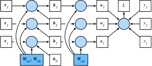
Vanilla RNNs model:
Computing the total prediction error in T steps:
Taking the derivatives with respect to
is fairly straightforward:
The dependency on
and
is a bit more tricky since it involves a chain of derivatives
After all, hidden states depend on each other and on past inputs:
Chaining terms together yields:
The Gradient has a long term dependency on the matrix .
有些场景下,RNNs模型仅使用最后一个状态的输出,此时
Vanishing and Exploding Gradients in Vanilla RNNs
RNNs suffer from the problem of vanishing and exploding gradients, which hampers learning of long data sequences. For example, the simplified RNN that does not take any input x, and not only computes the recurrence on the hidden state (equivalently the input x could always be zero):

The gradient signal going backwards in the time through all the hidden states is always being multiplied by the same matrix (the recurrence matrix ), interspersed with non-linearity backprop.
When you take one number and start multiplying it by some other number (i.e. a*b*b*b), this sequence either goes to zero if , or explodes to infinity when . The same thing happens in the backward pass of an RNN, expect is a matrix not just a number.
If the gradient vanishes it means the earlier hidden states have no real effect on the later hidden states, meaning no long term dependencies are learned! If the gradient explodes it mean the later hidden states is bigger and is difficult to learn!
There are a few ways to combat the vanishing gradient problem. Proper initialization of the W matrix can reduce the effect of vanishing gradients. A more preferred solution is to use ReLU instead of tanh or sigmoid activation functions. The ReLU derivative is a constant of either 0 or 1, so it isn’t as likely to suffer from vanishing gradients. An even more popular solution is to use Long Short-Term Memory (LSTM) or Gated Recurrent Unit (GRU) architectures.
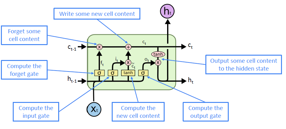
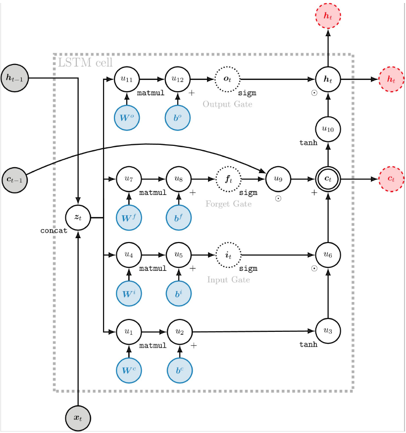
Long Short-Term Memory Networks, LSTMs
LSTM可解决RNN无法处理的长期依赖问题(梯度消失问题),通过三个Gate控制长期状态/记忆。
On timestep :
- forget gate:
- controls what parts of the previous cell state are written to cell state .
- input gate:
- controls what parts of the new cell state are written to cell state .
- output gate:
- controls what parts of cell state are output to hidden state.
- new cell content:
- new content to be written to the cell.
- cell state:
- erase (forget) some content from last cell state, and write (input) some new cell content.
- hidden state:
- read (output) some content from the cell, the length is same as
|
|
Preventing Vanishing Gradients with LSTMs
The biggest culprit in causing our gradients to vanish is that recursive derivative we need to compute: . If only this derivative was “well behaved” (that is, it doesn’t go to 0 or infinity as we back propagate through layers) then we could learn long term independencies!
The original LSTM solution
The original motivation behind the LSTM was to make this recursive derivative have a constant value, and then our gradients would neither explode or vanish.
The LSTM introduces a separate cell state
. In the original 1997 LSTM, the value for
depends on the previous value of the cell state and an update term weighted by the input gate value (see why):
This formulation doesn’t work well because the cell state tends to grow uncontrollably. In order to prevent this unbounded growth, a forget gate was added to scale the previous cell state, leading to the more modern formulation:
Looking at the full LSTM gradient
Let’s expand out the full derivation for
. First recall that in the LSTM,
is a function of
(the forget date),
(the input gate), and
(the candidate cell state), each of these being a function of
(since they are all functions of
). Via the multivariate chain rule we get:
Now if we want to backpropagate back k time steps, we simply multiply terms in the form of the one above k times. Note the big difference between this recursive gradient and the one for vanilla RNNs.
In vanilla RNNs, the terms will eventually take on a values that either always above 1 or always in the range [0, 1], this is essentially what leads to the vanishing/exploding gradient problem. The terms here, , at any time step can take on either values that are greater than 1 or values in the range [0, 1]. Thus if we extend to an infinite amount of time steps, it is not guaranteed that we will end up converging to 0 or infinity (unlike in vanilla RNNs).
If we start to converge to zero, we can always set the values of (lets say around 0.95 and other gate values) to be higher in order to bring the value of closer to 1, thus preventing the gradients from vanishing (or at the very least, preventing them from vanishing too quickly). One important thing to note is that the values and are things that the network learn to set. Thus, in this way the network learns to decide when to let the gradient vanish, and when to preserve it, by setting the gate values accordingly!
LSTM doesn’t guarantee that there is no vanishing/exploding gradient, but it does provide an easier way for the model to learn long-distance dependencies. This might all seem magical, but it really is just the result of two main things:
- The additive update function for the cell state gives a derivative that’s much more ‘well behaved’;
- The gating functions allow the network to decide how much the gradient vanishes, and can take on different values at each time step.
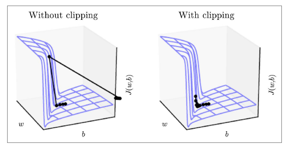
Gradient clipping: solution for exploding gradient
If the norm of the gradient is greater than some threshold, scale it down before applying SGD update
- If
then
- end if
This shows the loss surface a simple RNN (hidden state is scalar not a vector).
Gated Recurrent Units (GRU)
GRU as a simpler alternative to the LSTM. On each timestep , we have input and hidden state (no cell state).

On timestep :
- update gate:
- controls what parts of hidden state are updated vs preserved.
- reset gate:
- controls what parts of previous hidden state are used to compute new content.
- new hidden state content:
- selects useful parts of previous hidden state, combining current input to compute new hidden state.
- hidden state:
- simultaneously controls what is kept from previous hidden state, and what is updated to new hidden state content.
- is setting the balance between preserving things from the previous hidden state versus writing new stuff.
- is set to zero, then we’re going to be keeping the hidden state the same on every step, in order to retain information over long distances.
LSTM vs GRU
The biggest difference is that GRU is quicker to compute and has fewer parameters. There is no conclusive that one consistently performs better than the other.
Rule of thumb: start with LSTM, but switch to GRU if you want something more efficient. LSTM is a good default choice, especially if your data has particularly long dependencies, or you have lots of training data, because LSTM has more parameters than GRU that can learn more complex dependencies.
Vanishing/Exploding Gradient Solutions
Vanishing/exploding gradients are a general problem, RNNs are particularly unstable due to the repeated multiplication by the same weight matrix, for all neural architectures (including feed-forward and convolutional), especially deep ones.
- due to chain rule/choice of nonlinearity function, gradient can become vanishing small as it backpropagates;
- thus lower layers are learnt very slowly (hard to train);
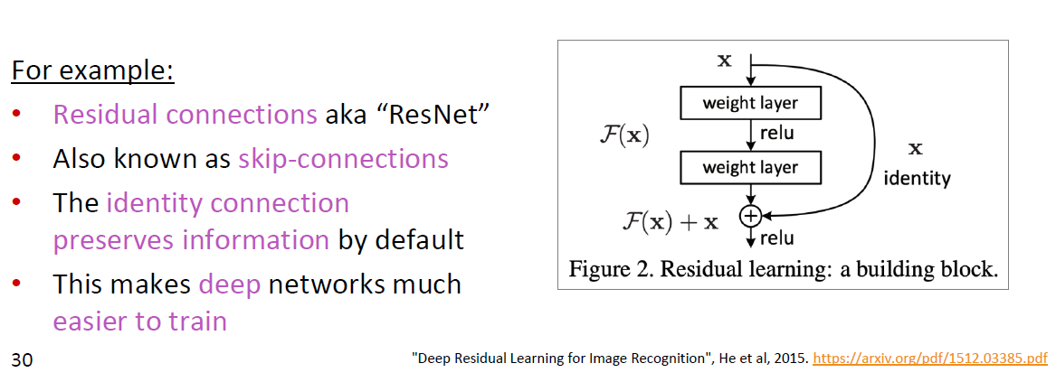
- solution: add more direct connections (thus allowing the gradient to flow);
Residual connections (ResNet)
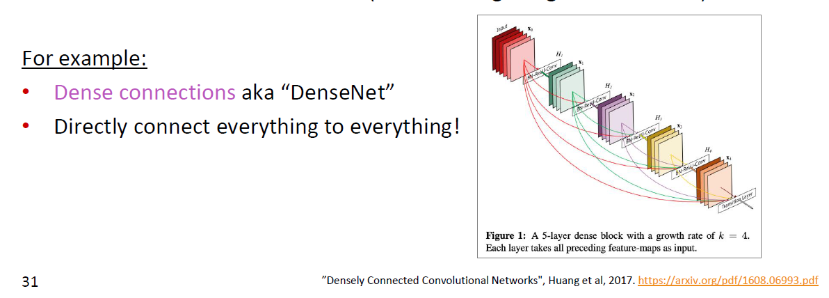
Dense connections (DenseNet)
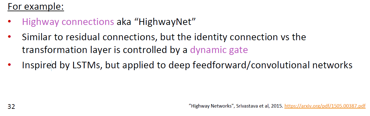
Highway connections (HighwayNet)
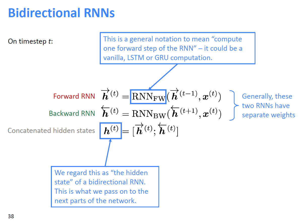
Bidirectional RNNs
Contextual representation of word by concatenating forward and backward RNN. There two RNNs have separate weights.
Multi-layer RNNs
Multi-layer RNNs are powerful, but you might need skip/dense-connections if it’s deep, such as BERT.
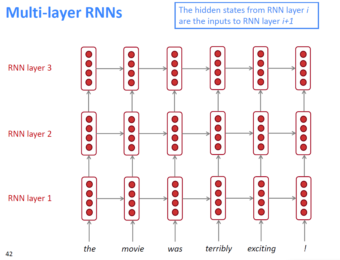
单向多层RNN可从前向后或从下(input)向上(output)学习,但是双向多层RNN只能从下向上学习.
Reference:
1. Why LSTMs Stop Your Gradients From Vanishing: A View from the Backwards Pass