Let
x
x
x
y
y
y
p
(
y
∣
x
;
w
)
=
exp
[
∑
j
=
1
J
w
j
F
j
(
x
,
y
)
]
Z
(
x
,
w
)
p(y | x ; w)=\frac{\exp [\sum_{j=1}^J w_{j} F_{j}(x, y)]}{Z(x, w)}
p ( y ∣ x ; w ) = Z ( x , w ) exp [ ∑ j = 1 J w j F j ( x , y ) ]
where the partition function
Z
(
x
,
w
)
=
∑
y
′
exp
[
∑
j
=
1
J
w
j
F
j
(
x
,
y
′
)
]
Z(x, w)=\sum_{y^{\prime}} \exp [\sum_{j=1}^J w_{j} F_{j}\left(x, y^{\prime}\right)]
Z ( x , w ) = y ′ ∑ exp [ j = 1 ∑ J w j F j ( x , y ′ ) ]
Note that in
∑
y
′
\sum_{y^{\prime}}
∑ y ′
y
y
y
x
x
x
y
^
=
argmax
y
p
(
y
∣
x
;
w
)
=
argmax
y
∑
j
=
1
J
w
j
F
j
(
x
,
y
)
\hat{y}=\underset{y}{\operatorname{argmax}} p(y | x ; w)=\underset{y}{\operatorname{argmax}} \sum_{j=1}^J w_{j} F_{j}(x, y)
y ^ = y a r g m a x p ( y ∣ x ; w ) = y a r g m a x j = 1 ∑ J w j F j ( x , y )
Each expression
F
j
(
x
,
y
)
F_j(x, y)
F j ( x , y )
j
j
j
(
x
,
y
)
(x,y)
( x , y )
Remark of the log-linear model:
a linear combination
∑
j
=
1
J
w
j
F
j
(
x
,
y
)
\sum_{j=1}^J w_{j} F_{j}(x, y)
∑ j = 1 J w j F j ( x , y )
The division makes the result
p
(
y
∣
x
;
w
)
p(y | x ; w)
p ( y ∣ x ; w )
Last time, we talked about Markov Random Fields. In this post, we are going to discuss Conditional Random Fields , which is an important special case of Markov Random Fields arises when they are applied to model a conditional probability distribution
p
(
y
∣
x
)
p(y|x)
p ( y ∣ x )
x
x
x
y
y
y
Formally, a CRF is a Markov network which specifies a conditional distribution
P
(
y
∣
x
)
=
1
Z
(
x
)
∏
c
∈
C
ϕ
c
(
x
c
,
y
c
)
P(y\mid x) = \frac{1}{Z(x)} \prod_{c \in C} \phi_c(x_c,y_c)
P ( y ∣ x ) = Z ( x ) 1 c ∈ C ∏ ϕ c ( x c , y c )
with partition function
Z
=
∑
y
∈
Y
∏
c
∈
C
ϕ
c
(
x
c
,
y
c
)
Z = \sum_{y \in \mathcal{Y}} \prod_{c \in C} \phi_c(x_c,y_c)
Z = y ∈ Y ∑ c ∈ C ∏ ϕ c ( x c , y c )
we further assume that the factors
ϕ
c
(
x
c
,
y
c
)
\phi_c(x_c,y_c)
ϕ c ( x c , y c )
ϕ
c
(
x
c
,
y
c
)
=
exp
[
w
c
T
f
c
(
x
c
,
y
c
)
]
\phi_c(x_c,y_c) = \exp[w_c^T f_c(x_c, y_c)]
ϕ c ( x c , y c ) = exp [ w c T f c ( x c , y c ) ]
Since we require our potential function
ϕ
\phi
ϕ
f
c
(
x
c
,
y
c
)
f_c(x_c, y_c)
f c ( x c , y c )
x
c
x_c
x c
y
c
y_c
y c etc .
As a remainder, let
x
x
x
y
y
y
p
(
y
∣
x
;
w
)
=
exp
[
∑
j
=
1
J
w
j
F
j
(
x
,
y
)
]
Z
(
x
,
w
)
p(y | x ; w)=\frac{\exp [\sum_{j=1}^J w_{j} F_{j}(x, y)]}{Z(x, w)}
p ( y ∣ x ; w ) = Z ( x , w ) exp [ ∑ j = 1 J w j F j ( x , y ) ]
From now on, we use the bar notation for sequences. Then to linear-CRF, we write the above equation as
p
(
y
ˉ
∣
x
ˉ
;
w
)
=
exp
[
∑
j
=
1
J
w
j
F
j
(
x
ˉ
,
y
ˉ
)
]
Z
(
x
ˉ
,
w
)
=
exp
[
∑
j
=
1
J
w
j
∑
i
=
2
T
f
j
(
y
i
−
1
,
y
i
,
x
ˉ
)
]
Z
(
x
ˉ
,
w
)
(
1
)
\begin{aligned} p(\bar y | \bar x; w) &= \frac{\exp [\sum_{j=1}^J w_{j} F_{j}(\bar x, \bar y)]}{Z(\bar x, w)}\\ &= \frac{\exp [\sum_{j=1}^J w_{j} \sum_{i=2}^{T} f_j (y_{i-1}, y_i, \bar x)]}{Z(\bar x, w)} &&\quad(1) \end{aligned}
p ( y ˉ ∣ x ˉ ; w ) = Z ( x ˉ , w ) exp [ ∑ j = 1 J w j F j ( x ˉ , y ˉ ) ] = Z ( x ˉ , w ) exp [ ∑ j = 1 J w j ∑ i = 2 T f j ( y i − 1 , y i , x ˉ ) ] ( 1 )
where
y
y
y
{
1
,
2
,
.
.
.
,
m
}
\{1,2,...,m\}
{ 1 , 2 , . . . , m }
Assume we have a sequence
x
ˉ
=
(
x
1
,
x
2
,
x
3
,
x
4
)
\bar x = (x_1, x_2, x_3, x_4)
x ˉ = ( x 1 , x 2 , x 3 , x 4 )
y
ˉ
=
(
y
1
,
y
2
,
y
3
,
y
4
)
\bar y = (y_1, y_2, y_3, y_4)
y ˉ = ( y 1 , y 2 , y 3 , y 4 )
We can divide each feature-function
F
j
(
x
ˉ
,
y
ˉ
)
F_j(\bar x, \bar y)
F j ( x ˉ , y ˉ )
F
j
(
x
ˉ
,
y
ˉ
)
=
∑
i
=
2
T
f
j
(
y
i
−
1
,
y
i
,
x
ˉ
)
(1.1)
F_j(\bar x, \bar y) = \sum_{i=2}^{T} f_j (y_{i-1}, y_i, \bar x) \tag {1.1}
F j ( x ˉ , y ˉ ) = i = 2 ∑ T f j ( y i − 1 , y i , x ˉ ) ( 1 . 1 )
Perticularly, from the above figure, since we have
3
3
3
F
j
(
x
ˉ
,
y
ˉ
)
=
f
j
(
y
1
,
y
2
,
x
ˉ
)
+
f
j
(
y
2
,
y
3
,
x
ˉ
)
+
f
j
(
y
3
,
y
4
,
x
ˉ
)
F_j(\bar x, \bar y) = f_j(y_1, y_2, \bar x) + f_j(y_2, y_3, \bar x) + f_j(y_3, y_4, \bar x)
F j ( x ˉ , y ˉ ) = f j ( y 1 , y 2 , x ˉ ) + f j ( y 2 , y 3 , x ˉ ) + f j ( y 3 , y 4 , x ˉ )
If we extract
J
J
J
(
x
ˉ
,
y
ˉ
)
(\bar x, \bar y)
( x ˉ , y ˉ )
∑
j
=
1
J
w
j
F
j
(
x
,
y
)
=
∑
j
=
1
J
w
j
∑
i
=
2
T
f
j
(
y
i
−
1
,
y
i
,
x
ˉ
)
\sum_{j=1}^J w_{j} F_{j}(x, y) = \sum_{j=1}^J w_{j} \sum_{i=2}^{T} f_j (y_{i-1}, y_i, \bar x)
j = 1 ∑ J w j F j ( x , y ) = j = 1 ∑ J w j i = 2 ∑ T f j ( y i − 1 , y i , x ˉ )
Goal: given a sequence
x
ˉ
\bar x
x ˉ
w
w
w
y
ˉ
\bar y
y ˉ
y
ˉ
\bar y
y ˉ
p
(
y
ˉ
∣
x
ˉ
;
w
)
=
exp
[
∑
j
=
1
J
w
j
∑
i
=
2
T
f
j
(
y
i
−
1
,
y
i
,
x
ˉ
)
]
Z
(
x
ˉ
,
w
)
p(\bar y | \bar x; w) = \frac{\exp [\sum_{j=1}^J w_{j} \sum_{i=2}^{T} f_j (y_{i-1}, y_i, \bar x)]}{Z(\bar x, w)}
p ( y ˉ ∣ x ˉ ; w ) = Z ( x ˉ , w ) exp [ ∑ j = 1 J w j ∑ i = 2 T f j ( y i − 1 , y i , x ˉ ) ]
Our objective is(check that the objective of CRF is the objective of Log-Linear model described above):
y
^
=
argmax
y
ˉ
p
(
y
ˉ
∣
x
ˉ
;
w
)
(
2
)
=
argmax
y
ˉ
∑
j
=
1
J
w
j
∑
i
=
2
T
f
j
(
y
i
−
1
,
y
i
,
x
ˉ
)
(
3
)
=
argmax
y
ˉ
∑
i
=
2
T
g
i
(
y
i
−
1
,
y
i
)
(
4
)
\begin{aligned} \hat{y} &= \underset{\bar y}{\operatorname{argmax}} p(\bar y | \bar x ; w) &&(2)\\ &= \underset{\bar y}{\operatorname{argmax}} \sum_{j=1}^J w_{j} \sum_{i=2}^{T} f_j (y_{i-1}, y_i, \bar x) &&(3) \\ &= \underset{\bar y}{\operatorname{argmax}} \sum_{i=2}^{T} g_i(y_{i-1}, y_i) && (4) \end{aligned}
y ^ = y ˉ a r g m a x p ( y ˉ ∣ x ˉ ; w ) = y ˉ a r g m a x j = 1 ∑ J w j i = 2 ∑ T f j ( y i − 1 , y i , x ˉ ) = y ˉ a r g m a x i = 2 ∑ T g i ( y i − 1 , y i ) ( 2 ) ( 3 ) ( 4 )
Note:
(
2
)
→
(
3
)
(2) \to (3)
( 2 ) → ( 3 )
y
ˉ
\bar y
y ˉ
We set
g
i
(
y
i
−
1
,
y
i
)
=
∑
j
=
1
J
w
j
⋅
f
j
(
y
i
−
1
,
y
i
,
x
ˉ
)
(5)
g_i(y_{i-1}, y_i) = \sum_{j=1}^J w_{j} \cdot f_j (y_{i-1}, y_i, \bar x) \tag 5
g i ( y i − 1 , y i ) = j = 1 ∑ J w j ⋅ f j ( y i − 1 , y i , x ˉ ) ( 5 )
Based on our objective in
(
5
)
(5)
( 5 )
y
1
y_1
y 1
y
T
y_T
y T Dynamic Programming (DP) here.
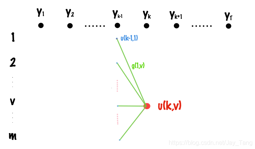
Let
u
(
k
,
v
)
u(k,v)
u ( k , v )
t
=
1
t=1
t = 1
t
=
k
t=k
t = k
k
k
k
v
v
v
u
(
k
,
v
)
=
max
s
[
u
(
k
−
1
,
s
)
+
g
k
(
s
,
v
)
]
u(k,v) = \underset{s}{\operatorname{max}} [u(k-1, s) + g_k(s,v)]
u ( k , v ) = s m a x [ u ( k − 1 , s ) + g k ( s , v ) ]
where
s
s
s
{
1
,
2
,
.
.
.
,
m
}
\{1,2,...,m\}
{ 1 , 2 , . . . , m }
max
{
u
(
T
,
1
)
,
u
(
T
,
2
)
,
.
.
.
,
u
(
T
,
m
)
}
\operatorname{max} \{u(T,1), u(T,2), ..., u(T,m)\}
m a x { u ( T , 1 ) , u ( T , 2 ) , . . . , u ( T , m ) }
Time complexity:
O
(
m
T
)
⋅
O
(
m
)
=
O
(
m
2
T
)
O(mT) \cdot O(m) = O(m^2 T)
O ( m T ) ⋅ O ( m ) = O ( m 2 T )
Space complexity:
O
(
m
T
)
O(mT)
O ( m T )
y
ˉ
\bar y
y ˉ
Goal: Given the data set
D
=
{
(
x
(
1
)
,
y
(
1
)
)
,
.
.
.
,
(
x
(
n
)
,
y
(
n
)
)
}
D = \{ ({x^{(1)}}, {y^{(1)}}), ..., ({x^{(n)}}, {y^{(n)}})\}
D = { ( x ( 1 ) , y ( 1 ) ) , . . . , ( x ( n ) , y ( n ) ) }
w
w
w
p
(
D
∣
w
)
p(D|w)
p ( D ∣ w )
w
^
M
L
E
=
max
w
p
(
D
∣
w
)
=
max
w
∏
i
=
1
n
p
(
y
(
i
)
∣
x
(
i
)
;
w
)
\begin{aligned} \hat{w}_{MLE} &= \underset{w}{\operatorname{max}} p(D|w) \\ &= \underset{w}{\operatorname{max}} \prod_{i=1}^{n} p( {y^{(i)}} | {x^{(i)}}; w) \end{aligned}
w ^ M L E = w m a x p ( D ∣ w ) = w m a x i = 1 ∏ n p ( y ( i ) ∣ x ( i ) ; w )
That is, we need to take derivatives and then use the gradient descent method.
p
(
y
ˉ
,
x
ˉ
;
w
)
=
exp
[
∑
j
=
1
J
w
j
F
j
(
x
,
y
)
]
Z
(
x
,
w
)
p(\bar y, \bar x; w) = \frac{\exp [\sum_{j=1}^J w_{j} F_{j}(x, y)]}{Z(x, w)}
p ( y ˉ , x ˉ ; w ) = Z ( x , w ) exp [ ∑ j = 1 J w j F j ( x , y ) ]
Take the derivative with respect to
w
j
w_j
w j
∂
∂
w
j
[
log
p
(
y
∣
x
;
w
)
]
=
∂
∂
w
j
[
∑
j
=
1
J
w
j
F
j
(
x
,
y
)
−
log
Z
(
x
,
w
)
]
=
F
j
(
x
,
y
)
−
1
Z
(
x
,
w
)
⋅
∂
∂
w
j
Z
(
x
,
w
)
(
6
)
\begin{aligned} \frac{\partial}{\partial w_j} [\log p(y| x; w)] &= \frac{\partial}{\partial w_j} [\sum_{j=1}^J w_{j} F_j(x, y) - \log Z(x,w)] \\ &= F_j(x, y) - \frac{1}{Z(x,w)} \cdot \frac{\partial}{\partial w_j} Z(x,w) &&(6) \end{aligned}
∂ w j ∂ [ log p ( y ∣ x ; w ) ] = ∂ w j ∂ [ j = 1 ∑ J w j F j ( x , y ) − log Z ( x , w ) ] = F j ( x , y ) − Z ( x , w ) 1 ⋅ ∂ w j ∂ Z ( x , w ) ( 6 )
where
∂
∂
w
j
Z
(
x
,
w
)
=
∂
∂
w
j
∑
y
′
exp
[
∑
j
=
1
J
w
j
F
j
(
x
,
y
′
)
]
=
∑
y
′
∂
∂
w
j
[
exp
∑
j
=
1
J
w
j
F
j
(
x
,
y
′
)
]
=
∑
y
′
[
exp
∑
j
=
1
J
w
j
F
j
(
x
,
y
′
)
]
⋅
F
j
(
x
,
y
′
)
(
7
)
\begin{aligned} \frac{\partial}{\partial w_j} Z(x,w) &= \frac{\partial}{\partial w_j} \sum_{y^{\prime}} \exp [\sum_{j=1}^J w_{j} F_{j}\left(x, y^{\prime}\right)] \\ &= \sum_{y^{\prime}} \frac{\partial}{\partial w_j} [\exp \sum_{j=1}^J w_{j} F_{j}\left(x, y^{\prime}\right)] \\ &= \sum_{y^{\prime}} [\exp \sum_{j=1}^J w_{j} F_{j}\left(x, y^{\prime}\right)] \cdot F_{j}\left(x, y^{\prime}\right) &&(7) \end{aligned}
∂ w j ∂ Z ( x , w ) = ∂ w j ∂ y ′ ∑ exp [ j = 1 ∑ J w j F j ( x , y ′ ) ] = y ′ ∑ ∂ w j ∂ [ exp j = 1 ∑ J w j F j ( x , y ′ ) ] = y ′ ∑ [ exp j = 1 ∑ J w j F j ( x , y ′ ) ] ⋅ F j ( x , y ′ ) ( 7 )
Combining
(
6
)
(6)
( 6 )
(
7
)
(7)
( 7 )
∂
∂
w
j
[
log
p
(
y
∣
x
;
w
)
]
=
F
j
(
x
,
y
)
−
1
Z
(
x
,
w
)
∑
y
′
F
j
(
x
,
y
′
)
[
exp
∑
j
=
1
J
w
j
F
j
(
x
,
y
′
)
]
=
F
j
(
x
,
y
)
−
∑
y
′
F
j
(
x
,
y
′
)
exp
∑
j
=
1
J
w
j
F
j
(
x
,
y
′
)
Z
(
x
,
w
)
=
F
j
(
x
,
y
)
−
∑
y
′
F
j
(
x
,
y
′
)
⋅
p
(
y
′
∣
x
;
w
)
=
F
j
(
x
,
y
)
−
E
y
′
∼
p
(
y
′
∣
x
;
w
)
[
F
j
(
x
,
y
′
)
]
(
8
)
\begin{aligned} \frac{\partial}{\partial w_j} [\log p(y| x; w)] &= F_{j}\left(x, y\right) - \frac{1}{Z(x,w)} \sum_{y^{\prime}} F_{j}\left(x, y^{\prime}\right) [\exp \sum_{j=1}^J w_{j} F_{j}\left(x, y^{\prime}\right)] \\ &= F_{j}\left(x, y\right) - \sum_{y^{\prime}} F_{j}\left(x, y^{\prime}\right) \frac{\exp \sum_{j=1}^J w_{j} F_{j}\left(x, y^{\prime}\right)}{Z(x,w)} \\ &= F_{j}\left(x, y\right) - \sum_{y^{\prime}} F_{j}\left(x, y^{\prime}\right) \cdot p(y^{\prime}|x;w) \\ &= F_{j}\left(x, y\right) - E_{y^{\prime} \sim p(y^{\prime}|x;w)}[F_{j}\left(x, y^{\prime}\right)] &&(8) \end{aligned}
∂ w j ∂ [ log p ( y ∣ x ; w ) ] = F j ( x , y ) − Z ( x , w ) 1 y ′ ∑ F j ( x , y ′ ) [ exp j = 1 ∑ J w j F j ( x , y ′ ) ] = F j ( x , y ) − y ′ ∑ F j ( x , y ′ ) Z ( x , w ) exp ∑ j = 1 J w j F j ( x , y ′ ) = F j ( x , y ) − y ′ ∑ F j ( x , y ′ ) ⋅ p ( y ′ ∣ x ; w ) = F j ( x , y ) − E y ′ ∼ p ( y ′ ∣ x ; w ) [ F j ( x , y ′ ) ] ( 8 )
We can edit
(
8
)
(8)
( 8 )
∂
∂
w
j
[
log
p
(
y
ˉ
∣
x
ˉ
;
w
)
]
=
F
j
(
x
ˉ
,
y
ˉ
)
−
E
y
ˉ
′
∼
p
(
y
ˉ
′
∣
x
;
w
)
[
F
j
(
x
,
y
ˉ
′
)
]
(
9
)
=
F
j
(
x
ˉ
,
y
ˉ
)
−
E
y
ˉ
′
[
∑
i
=
2
T
f
j
(
y
i
−
1
,
y
i
,
x
ˉ
)
]
(
10
)
=
F
j
(
x
ˉ
,
y
ˉ
)
−
∑
i
=
2
T
E
y
ˉ
′
[
f
j
(
y
i
−
1
,
y
i
,
x
ˉ
)
]
(
11
)
=
F
j
(
x
ˉ
,
y
ˉ
)
−
∑
i
=
2
T
E
y
i
−
1
,
y
i
[
f
j
(
y
i
−
1
,
y
i
,
x
ˉ
)
]
(
12
)
=
F
j
(
x
ˉ
,
y
ˉ
)
−
∑
i
=
2
T
∑
y
i
−
1
∑
y
i
f
j
(
y
i
−
1
,
y
i
,
x
ˉ
)
⋅
p
(
y
i
−
1
,
y
i
∣
x
ˉ
;
w
)
(
13
)
\begin{aligned} \frac{\partial}{\partial w_j} [\log p(\bar y| \bar x; w)] &= F_{j}\left(\bar x, \bar y\right) - E_{\bar y^{\prime} \sim p(\bar y^{\prime}|x;w)}[F_{j}\left(x,\bar y^{\prime}\right)] &&(9)\\ &= F_{j}\left(\bar x, \bar y\right) - E_{\bar y^{\prime}}[\sum_{i=2}^T f_j(y_{i-1}, y_i, \bar x)] &&(10)\\ &= F_{j}\left(\bar x, \bar y\right) - \sum_{i=2}^T E_{\bar y^{\prime} }[f_j(y_{i-1}, y_i, \bar x)] &&(11)\\ &= F_{j}\left(\bar x, \bar y\right) - \sum_{i=2}^T E_{y_{i-1}, y_i}[f_j(y_{i-1}, y_i, \bar x)] &&(12)\\ &= F_{j}\left(\bar x, \bar y\right) - \sum_{i=2}^T \sum_{y_{i-1}} \sum_{y_{i}} f_j(y_{i-1}, y_i, \bar x) \cdot p(y_{i-1}, y_i| \bar x; w) &&(13) \end{aligned}
∂ w j ∂ [ log p ( y ˉ ∣ x ˉ ; w ) ] = F j ( x ˉ , y ˉ ) − E y ˉ ′ ∼ p ( y ˉ ′ ∣ x ; w ) [ F j ( x , y ˉ ′ ) ] = F j ( x ˉ , y ˉ ) − E y ˉ ′ [ i = 2 ∑ T f j ( y i − 1 , y i , x ˉ ) ] = F j ( x ˉ , y ˉ ) − i = 2 ∑ T E y ˉ ′ [ f j ( y i − 1 , y i , x ˉ ) ] = F j ( x ˉ , y ˉ ) − i = 2 ∑ T E y i − 1 , y i [ f j ( y i − 1 , y i , x ˉ ) ] = F j ( x ˉ , y ˉ ) − i = 2 ∑ T y i − 1 ∑ y i ∑ f j ( y i − 1 , y i , x ˉ ) ⋅ p ( y i − 1 , y i ∣ x ˉ ; w ) ( 9 ) ( 1 0 ) ( 1 1 ) ( 1 2 ) ( 1 3 )
Note:
(
9
)
→
(
10
)
(9) \to (10)
( 9 ) → ( 1 0 )
(
1
)
(1)
( 1 )
(
11
)
→
(
12
)
(11) \to (12)
( 1 1 ) → ( 1 2 )
f
j
(
y
i
−
1
,
y
i
,
x
ˉ
)
f_j(y_{i-1}, y_i, \bar x)
f j ( y i − 1 , y i , x ˉ )
y
i
−
1
y_{i-1}
y i − 1
y
i
y_i
y i
In the equation
(
13
)
(13)
( 1 3 )
p
(
y
i
−
1
,
y
i
∣
x
ˉ
;
w
)
p(y_{i-1}, y_i| \bar x; w)
p ( y i − 1 , y i ∣ x ˉ ; w )
Z
(
x
ˉ
,
w
)
Z(\bar x, w)
Z ( x ˉ , w )
Z
(
x
ˉ
,
w
)
=
∑
y
ˉ
exp
[
∑
j
=
1
J
w
j
F
j
(
x
ˉ
,
y
ˉ
)
]
=
∑
y
ˉ
exp
[
∑
j
=
1
J
w
j
∑
i
=
2
T
f
j
(
y
i
−
1
,
y
i
,
x
ˉ
)
]
=
∑
y
ˉ
[
exp
∑
i
=
2
T
g
i
(
y
i
−
1
,
y
i
)
]
(
14
)
\begin{aligned} Z(\bar x, w) &= \sum_{\bar y} \exp \left[\sum_{j=1}^J w_{j} F_{j}\left(\bar x, \bar y \right)\right] \\ &= \sum_{\bar y} \exp \left[\sum_{j=1}^J w_{j} \sum_{i=2}^T f_j(y_{i-1}, y_i, \bar x)\right] \\ &= \sum_{\bar y} \left[\exp \sum_{i=2}^T g_i(y_{i-1}, y_i)\right] && (14) \end{aligned}
Z ( x ˉ , w ) = y ˉ ∑ exp [ j = 1 ∑ J w j F j ( x ˉ , y ˉ ) ] = y ˉ ∑ exp [ j = 1 ∑ J w j i = 2 ∑ T f j ( y i − 1 , y i , x ˉ ) ] = y ˉ ∑ [ exp i = 2 ∑ T g i ( y i − 1 , y i ) ] ( 1 4 )
We see the term
g
i
(
y
i
−
1
,
y
i
)
g_i(y_{i-1}, y_i)
g i ( y i − 1 , y i )
(
14
)
(14)
( 1 4 )
(
14
)
(14)
( 1 4 )
[
exp
∑
i
=
2
T
g
i
(
y
i
−
1
,
y
i
)
]
\left[\exp \sum_{i=2}^T g_i(y_{i-1}, y_i)\right]
[ exp ∑ i = 2 T g i ( y i − 1 , y i ) ]
y
y
y
O
(
m
T
)
O(m^T)
O ( m T ) forward algorithm and backward algorithm . Note that this is very similar to HMM we discussed before.
Let
α
(
k
,
v
)
\alpha(k,v)
α ( k , v )
t
=
1
t=1
t = 1
t
=
k
t=k
t = k
k
k
k
v
v
v
α
(
k
,
v
)
=
max
s
[
α
(
k
−
1
,
s
)
⋅
exp
g
k
(
s
,
v
)
]
\alpha(k,v) = \underset{s}{\operatorname{max}} \left[\alpha(k-1, s) \cdot \text{exp}\, g_k(s,v)\right]
α ( k , v ) = s m a x [ α ( k − 1 , s ) ⋅ exp g k ( s , v ) ]
where
s
∈
{
1
,
2
,
.
.
.
,
m
}
s \in \{1,2,...,m\}
s ∈ { 1 , 2 , . . . , m }
Z
(
x
ˉ
,
w
)
Z(\bar x, w)
Z ( x ˉ , w )
Z
(
x
ˉ
,
w
)
=
∑
s
=
1
m
α
(
T
,
s
)
Z(\bar x, w) = \sum_{s=1}^m \alpha(T, s)
Z ( x ˉ , w ) = s = 1 ∑ m α ( T , s )
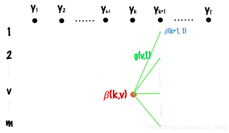
Let
β
(
k
,
v
)
\beta(k,v)
β ( k , v )
t
=
k
t=k
t = k
t
=
T
t=T
t = T
t
t
t
v
v
v
β
(
k
,
v
)
=
max
s
[
β
(
k
+
1
,
s
)
⋅
exp
g
k
+
1
(
v
,
s
)
]
\beta(k,v) = \underset{s}{\operatorname{max}} \left[\beta(k+1, s) \cdot \text{exp}\, g_{k+1}(v,s)\right]
β ( k , v ) = s m a x [ β ( k + 1 , s ) ⋅ exp g k + 1 ( v , s ) ]
where
s
∈
{
1
,
2
,
.
.
.
,
m
}
s \in \{1,2,...,m\}
s ∈ { 1 , 2 , . . . , m }
Z
(
x
ˉ
,
w
)
Z(\bar x, w)
Z ( x ˉ , w )
Z
(
x
ˉ
,
w
)
=
∑
s
=
1
m
β
(
1
,
s
)
Z(\bar x, w) = \sum_{s=1}^m \beta(1, s)
Z ( x ˉ , w ) = s = 1 ∑ m β ( 1 , s )
p
(
y
k
=
u
∣
x
ˉ
;
w
)
p(y_k=u|\bar x; w)
p ( y k = u ∣ x ˉ ; w ) From the figure above, we can divide it into the product of a forward term and a backward term:
p
(
y
k
=
u
∣
x
ˉ
;
w
)
=
α
(
k
,
u
)
⋅
β
(
k
,
u
)
Z
(
x
ˉ
,
w
)
p(y_k=u|\bar x; w) = \frac{\alpha(k,u)\cdot \beta(k,u)}{Z(\bar x, w)}
p ( y k = u ∣ x ˉ ; w ) = Z ( x ˉ , w ) α ( k , u ) ⋅ β ( k , u )
where
Z
(
x
ˉ
,
w
)
=
∑
u
α
(
k
,
u
)
⋅
β
(
k
,
u
)
Z(\bar x, w) = \sum_u \alpha(k,u)\cdot \beta(k,u)
Z ( x ˉ , w ) = u ∑ α ( k , u ) ⋅ β ( k , u )
Note that we can also compute
Z
(
x
ˉ
,
w
)
Z(\bar x, w)
Z ( x ˉ , w )
α
\alpha
α
β
\beta
β
p
(
y
k
=
u
,
y
k
+
1
=
v
∣
x
ˉ
;
w
)
p(y_k=u, y_{k+1}=v|\bar x; w)
p ( y k = u , y k + 1 = v ∣ x ˉ ; w ) From the figure above, we can divide it into the product of a forward term, a backward term, and an term that represent the path going from
y
k
=
u
y_k=u
y k = u
y
k
+
1
=
v
y_{k+1}= v
y k + 1 = v
p
(
y
k
=
u
,
y
k
+
1
=
v
∣
x
ˉ
;
w
)
=
α
(
k
,
u
)
⋅
[
exp
g
k
+
1
(
u
,
v
)
]
⋅
β
(
k
+
1
,
v
)
Z
(
x
ˉ
,
w
)
p(y_k=u, y_{k+1}=v|\bar x; w) = \frac{\alpha(k,u)\cdot [\text{exp} \, g_{k+1} (u,v)] \cdot\beta(k+1,v)}{Z(\bar x, w)}
p ( y k = u , y k + 1 = v ∣ x ˉ ; w ) = Z ( x ˉ , w ) α ( k , u ) ⋅ [ exp g k + 1 ( u , v ) ] ⋅ β ( k + 1 , v )
where
Z
(
x
ˉ
,
w
)
=
∑
u
∑
v
α
(
k
,
u
)
⋅
[
exp
g
k
+
1
(
u
,
v
)
]
⋅
β
(
k
+
1
,
v
)
Z(\bar x, w) = \sum_u \sum_v \alpha(k,u)\cdot [\text{exp} \, g_{k+1} (u,v)] \cdot\beta(k+1,v)
Z ( x ˉ , w ) = u ∑ v ∑ α ( k , u ) ⋅ [ exp g k + 1 ( u , v ) ] ⋅ β ( k + 1 , v )
Now go back to where we stopped (equation
(
13
)
(13)
( 1 3 )
∂
∂
w
j
[
log
p
(
y
ˉ
∣
x
ˉ
;
w
)
]
=
F
j
(
x
ˉ
,
y
ˉ
)
−
∑
i
=
2
T
∑
y
i
−
1
∑
y
i
f
j
(
y
i
−
1
,
y
i
,
x
ˉ
)
⋅
p
(
y
i
−
1
,
y
i
∣
x
ˉ
;
w
)
=
F
j
(
x
ˉ
,
y
ˉ
)
−
∑
i
=
2
T
∑
y
i
−
1
∑
y
i
f
j
(
y
i
−
1
,
y
i
,
x
ˉ
)
⋅
α
(
i
−
1
,
y
i
−
1
)
⋅
[
exp
g
i
(
y
i
−
1
,
y
i
)
]
⋅
β
(
i
,
y
1
)
Z
(
x
ˉ
,
w
)
(
15
)
\begin{aligned} \frac{\partial}{\partial w_j} [\log p(\bar y| \bar x; w)] &= F_{j}\left(\bar x, \bar y\right) - \sum_{i=2}^T \sum_{y_{i-1}} \sum_{y_{i}} f_j(y_{i-1}, y_i, \bar x) \cdot p(y_{i-1}, y_i| \bar x; w) \\ &= F_{j}\left(\bar x, \bar y\right) - \sum_{i=2}^T \sum_{y_{i-1}} \sum_{y_{i}} f_j(y_{i-1}, y_i, \bar x) \cdot \frac{\alpha(i-1,y_{i-1})\cdot [\text{exp} \, g_{i} (y_{i-1},y_i)] \cdot\beta(i,y_1)}{Z(\bar x, w)} &&(15) \end{aligned}
∂ w j ∂ [ log p ( y ˉ ∣ x ˉ ; w ) ] = F j ( x ˉ , y ˉ ) − i = 2 ∑ T y i − 1 ∑ y i ∑ f j ( y i − 1 , y i , x ˉ ) ⋅ p ( y i − 1 , y i ∣ x ˉ ; w ) = F j ( x ˉ , y ˉ ) − i = 2 ∑ T y i − 1 ∑ y i ∑ f j ( y i − 1 , y i , x ˉ ) ⋅ Z ( x ˉ , w ) α ( i − 1 , y i − 1 ) ⋅ [ exp g i ( y i − 1 , y i ) ] ⋅ β ( i , y 1 ) ( 1 5 )
Now every term in the equation
(
15
)
(15)
( 1 5 )
w
w
w
Reference:
https://ermongroup.github.io/cs228-notes/representation/undirected/
http://cseweb.ucsd.edu/~elkan/250B/CRFs.pdf
http://homepages.inf.ed.ac.uk/csutton/publications/crftut-fnt.pdf
http://cseweb.ucsd.edu/~elkan/250Bfall2007/loglinear.pdf