梯度提升机（Gradient Boosting Machine）之 XGBoost

XGBoost 学习总结

相对于随机森林使用 bagging 融合完全长成决策树，梯度提升决策树使用的 boosting 的改进版本 AdaBoost 技术的广义版本，也就是说是根据损失函数的梯度方向，所以叫做梯度提升（Gradient Boosting）。

XGBoost 实际上就是对全部的决策树输出取加权平均，加权值为衰减系数或者1。当前 k - 1 颗树已经训练好时，对 k 颗树集成后的损失函数取二阶泰勒展开（在前 k - 1 颗树的集成模型处），便可以根据一阶导数和二阶导数求出最佳的解和目标值，但是前提是已知最佳的分组。这里最佳的分组的获取分为两个部分：当前特征维度上的最佳分割点、全部特征中的最佳分割特征。那么单个特征维度上的最佳分割点是通过对当前分支上全部的样本根据该特征进行排序，然后从头到尾穷举寻找到最佳分割点。最佳分割特征则是根据特征的最佳目标值获取全部特征中的最佳特征。由于穷举是很费时间的，所以这里也采用一种分桶操作提高效率，做分桶时是根据二阶导数对当前特征值排序后，再按分位数进行分桶的。

下面进行详细的分析：

常用的数学符号（Basic Notations）

假设叶子节点的排列顺序是从左到右，使用 $w^{(k)}_m$ 表示第 k 颗树的第 t 个叶子节点的值，假如全部的叶子节点个数为 $T$，那么第 k 颗树的全部叶子节点的向量表示为：

$w^{(k)} = (w^{(k)}_1,w^{(k)}_2,\cdots,w^{(k)}_K)$

为了推导简单下文中使用 $w$ 代表 $w^{(k)}$ 即最后一颗树的权重向量。

同时使用 $q^{(k)} ( x_i )$ 代表样本 $x_i$ 所在叶子节点的位置。为了推导简单下文中使用 $q ( x_i )$ 代表 $q^{(k)} ( x_i )$ 即最后一颗树的样本位置。即 $w_{q ( x_i )}$ 代表了样本 $x_i$ 对应的第 k 颗树的预测值 $f _ { k } \left( x _ { i } \right)$。

另外使用集合 $I^{(k)} _ { t }$ 表示所在第 k 颗树的第 t 个节点的全部样本集合。

$I ^{(k)}_ { t } = \left\{ x_i | q^{(k)} \left( { x } _ { i } \right) = { t } \right\}$

为了推导简单下文中使用 $I _ { j }$ 表示 $I ^{(k)}_ { j }$。即最后一颗树的样本分布集合

正则化学习目标（Regularized Learning Objective）

给定一个有 n 个样本和 m 个特征的数据集 $\mathcal { D } = \left\{ \left( \mathbf { x } _ { i } , y _ { i } \right) \right\} \left( | \mathcal { D } | = n , \mathbf { x } _ { i } \in \mathbb { R } ^ { m } , y _ { i } \in \mathbb { R } \right)$，假设第 k 棵树的预测函数（Hypothesis）为： $f _ { k } \left( x _ { i } \right)$，那么在XGBoost中，使用 K 棵树集成模型的的第 i 个样本的预测值为 $\hat { y } _ { i }$：

$\hat { y } _ { i } = \phi \left( \mathbf { x } _ { i } \right) = \sum _ { k = 1 } ^ { K } f _ { k } \left( \mathbf { x } _ { i } \right) , \quad f _ { k } \in \mathcal { F }$

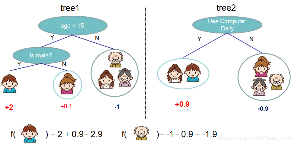
该集成方法以下图为例：

可以看出与广义的 GBDT 不同的地方是其系数是 1 。

可以看出这是一种 Additive Training(叠加式的训练)，因为其本身也是一种 GBDT，所以其训练过程也是需要使用前一个 hypothesis 的预测余数进行下一个 hypothesis 的获取的。也就是说其每颗树模型的预测值可以做如下传递：

$\begin{aligned} \hat { y } _ { i } ^ { ( 0 ) } & = 0 \quad \leftarrow \quad \text { Default case } \\ \hat { y } _ { i } ^ { ( 1 ) } &= f _ { 1 } \left( x _ { j } \right) = \hat { y } _ { i } ^ { 0} + f _ { 1 } \left( x _ { i } \right) \\ \hat { y } _ { i } ^ { ( 2 ) } & = f _ { 1 } \left( x _ { i } \right) + f _ { 2 } \left( x _ { 0 } \right) = \hat { y } _ { i } ^ { ( 2 ) } + f _ { 2 } \left( x _ { 2 } \right) \\ & \, \, \, \vdots \\ \hat { y } _ { i } ^ { ( k ) } &= { f _ { 1 } \left( x _ { 0 } \right) + f _ { 2 } \left( x _ { i } \right) + \cdots + f _ { k } \left( x _ { i } \right) } \\& = { \sum _ { j = 1 } ^ { (k-1)} f _ { j } \left( x _ { i } \right) + f _ { k } \left( x _ { i } \right) } = \hat { y } _ { i } ^ { ( k - 1 ) } + f _ { k } \left( x _ { i } \right) \end{aligned}$

加入正则化项后的目标函数可以写为：

$\mathcal { L } ( \phi ) =\underbrace { \sum _ { i = 1 } ^ { n } l \left( y _ { i } , \widehat { y } _ { i } \right)}_ \text { Loss Function }+ \underbrace { \sqrt { \sum _ { k = 1 } ^ { K } \Omega \left( f _ { k } \right) } } _ \text{ Penalty/Regularization }$

其中损失函数可以任意选择，正则化项为：

$\Omega \left( f _ { k } \right) = \gamma T + \frac{1}{2} \lambda \sum _ { t = 1 } ^ { T } \left(w _ { t} \right) ^ { 2 }$

这里使用叶子节点的个数和参数的 L2 范数相结合，正则化项的加入是为了帮助使得最终学习到的权重比较平滑而不会过拟合（ The additional regularization term helps to smooth the final learnt weights to avoid over-fitting.）针对决策树而言，正则化操作一般是控制叶子的节点个数，树的深度，叶子的节点值。

当然除却正则化项的加入，也引入了放缩（Shrinkage，对每代生成的树赋予权重系数 $\eta$，即 $\hat { \boldsymbol { y } } _ { i } ^ { t } = \hat { \boldsymbol { y } } _ { i } ^ { ( t - 1 ) } + \eta \boldsymbol { f } _ { t } \left( \boldsymbol { x } _ { i } \right)$）和列子集采样（Column Subsampling，随机选择选取 $d^{\prime}$ 个特征，其中 $d^{\prime} \leq d$，即使用一部分特征训练）技术来防止过拟合，

梯度提升树（Gradient Tree Boosting）

根据叠加式训练的特点目标函数可以改写为：

$\begin{aligned} \mathcal { L } ^ { ( k ) } &= \sum _ { i = 1 } ^ { n } l \left( y _ { i } , \hat { y } _ { i } ^ { ( k - 1 ) } + f _ { t } \left( \mathbf { x } _ { i } \right) \right) + \Omega \left( f _ { t } \right) \\ &= \sum _ { i = 1 } ^ { n } l \left( y _ { i } , \hat { y } _ { i } ^ { ( k - 1 ) } + f _ { k } \left( \mathbf x _ { i } \right)\right) + \sum _ { j = 1 } ^ { k - 1 } \Omega \left( f _ { j } \right) + \Omega \left( f _ { k } \right) \end{aligned}$

其中由于 $\sum _ { j = 1 } ^ { k - 1 } \Omega \left( f _ { j } \right)$ 是常值，所以该最优化问题可以写为：

$\operatorname{minimize } \sum _ { i = 1 } ^ { n } l \left( y _ { i } , \hat { y } _ { i } ^ { ( k - 1 ) } + f _ { k } \left( \mathbf x _ { i } \right)\right) + \Omega \left( f _ { k } \right)$

知识回顾

泰勒级数
$\begin{aligned} & f(x+\Delta x) \\= &f \left( x \right) + f ^ { \prime } \left( x \right) \left( \Delta x \right) + \frac { f ^ { \prime \prime } \left( x \right) } { 2 ! } \left( \Delta x \right) ^ { 2 } + \cdots + \frac { f ^ { ( n ) } \left( x \right) } { n ! } \left( \Delta x \right) ^ { n } + \cdots \\=&\sum _ { n = 0 } ^ { \infty } \frac { f ^ { ( n ) } \left( x \right) } { n ! } \left( \Delta x \right) ^ { n } \end{aligned}$

为了方便求解，对目标函数进行二阶泰勒展开（将常数项抽取出来），对比与泰勒展开式，这里将常数 $\hat { y } _ { i } ^ { ( k - 1 ) }$ 视作 $x$，将 $f _ { k } \left( \mathbf x _ { i } \right)$ 视作 $\Delta x$：

$f ( x + \Delta x ) = l \left( y _ { i } , \underbrace{ \hat { y } _ { i } ^ { ( k - 1 ) } }_{x}+ \underbrace{ f _ { k } \left( \mathbf x _ { i } \right)}_{\Delta x} \right)$

目标函数的二阶泰勒展开为：

$\begin{aligned} & \sum _ { i = 1 } ^ { n } l \left( y _ { i } , \hat { y } _ { i } ^ { ( k - 1 ) } + f _ { k } \left( \mathbf x _ { i } \right)\right) + \Omega \left( f _ { k } \right) \\ = & \sum _ { i = 1 } ^ { n } \left[ l \left( y _ { i } , \hat { y } _ { i } ^ { ( k - 1 ) } \right) + l^{\prime} \left( y _ { i } , \hat { y } _ { i } ^ { ( k - 1 ) } \right) f _ { k } \left( \mathbf x _ { i } \right) + \frac{1}{2} l^{\prime\prime} \left( y _ { i } , \hat { y } _ { i } ^ { ( k - 1 ) } \right) f^{2} _ { k } \left( \mathbf x _ { i } \right) \right]+ \Omega \left( f _ { k } \right)\\ = & \sum _ { i = 1 } ^ { n } \left[ l \left( y _ { i } , \hat { y } _ { i } ^ { ( k - 1 ) } \right) + g_i f _ { k } \left( \mathbf x _ { i } \right) + \frac{1}{2} h_i f^{2} _ { k } \left( \mathbf x _ { i } \right) \right]+ \Omega \left( f _ { k } \right) \Leftarrow l^{\prime} \left( y _ { i } , \hat { y } _ { i } ^ { ( k - 1 ) } \right),l^{\prime\prime} \left( y _ { i } , \hat { y } _ { i } ^ { ( k - 1 ) } \right) \rightarrow g_i,h_i\\ \end{aligned}$

那么在训练第 k 个基模型时， $l \left( y _ { i } , \hat { y } _ { i } ^ { ( k - 1 ) } \right) ,g_i,h_i$ 是已知的，可以视为常值。

那么该最优化问题可以进一步改写为：

$\operatorname{minimize } \sum _ { i = 1 } ^ { n } \left[g_i f _ { k } \left( \mathbf x _ { i } \right) + \frac{1}{2} h_i f^{2} _ { k } \left( \mathbf x _ { i } \right) \right]+ \Omega \left( f _ { k } \right)$

那么参数化后的新目标函数可以写为：

$\begin{aligned} & \sum _ { i = 1 } ^ { n } \left[ g_i f _ { k } \left( \mathbf x _ { i } \right) + \frac{1}{2} h_i f^{2} _ { k } \left( \mathbf x _ { i } \right) \right]+ \Omega \left( f _ { k } \right) \\ = & \sum _ { i = 1 } ^ { n } \left[ g_i w_{q ( \mathbf x_i )} + \frac{1}{2} h_i {w^{2}_{q ( \mathbf x_i )}} \right]+ \gamma T + \frac{1}{2} \lambda \sum _ { t = 1 } ^ { T } \left(w _ { t} \right) ^ { 2 } \\ = & \sum _ { t = 1 } ^ { T } \left[ \underbrace{\sum _ { i \in I _ { t } } g_i }_{\text{constant } G_t } w_{t} + \frac{1}{2} (\underbrace{\sum _ { i \in I _ { t } } h_i }_{\text{constant } H_t } + \lambda ){w^{2}_{t}}\right]+ \gamma T \\ \end{aligned}$

那么在中括号中，由于 $G_t,H_t$ 是常值，所以是一个关于 $w_t$ 二次函数求最优解问题。

知识回顾：

一个典型的二次函数：
$y = a x ^ { 2 } + b x + c \quad ( a \neq 0 )$
其最小值点为
$\left( - \frac { b } { 2 a } , \frac { 4 a c - b ^ { 2 } } { 4 a } \right)$

所以当树的结构固定，也就是说 $q(\mathbf x)$ 固定的话，在中括号中的最佳 $w^*_t$ 为：

$-\frac{G_t}{H_t + \lambda}$

括号中的最佳解（最小值）为：

$-\frac{G_t^2}{ 2(H_t + \lambda)}$

所以当前树结构下的最佳的目标函数值 $\mathcal { L } ^ *$ 为：

$-\frac{1}{2} \sum _ { t = 1 } ^ { T } \frac{G_t^2}{ H_t + \lambda} + \gamma T$

以下图为例计算目标函数函数值：

寻找分割算法（Split Finding Algorithm）

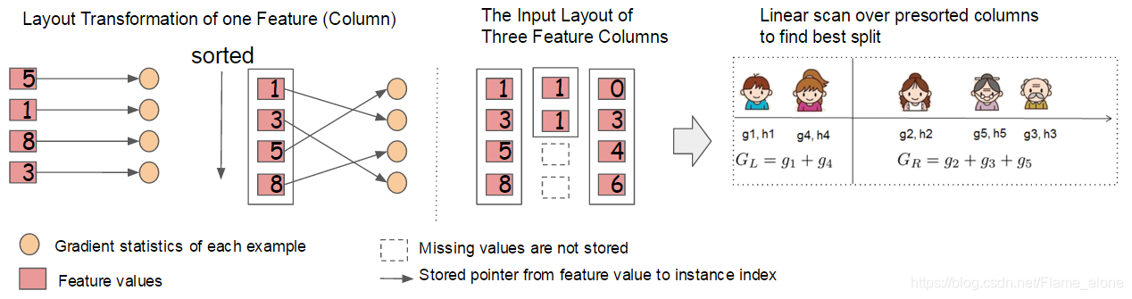
精确贪心算法表明，对于连续特征，计算上要求枚举所有可能的分割。为了有效地实现这一点，算法必须首先根据特征值对数据进行排序，然后访问排序后的数据，以实现最佳分割点的获取。（因为排序之后数据集的分割会高效很多，可以直接在原内存上直接读取使用）

分割点估计算法（Approximate Algorithm for Split Finding）

既然可以计算出最佳的目标值，那么假设当前节点的样本集为 $I = I _ { L } \cup I _ { R }$，其中 $I _ { L } , I _ { R }$ 分别为分割后左子树和右子树分别分的样本集，那么分割后的损失（目标）函数将减少：

$\mathcal { L } _\text{split} = \frac { 1 } { 2 } \left[ \frac { G _ { L } ^ { 2 } } { H _ { L + \lambda } } + \frac { G _ { R } ^ { 2 } } { H _ { R } + \lambda } - \frac { \left( G_L + G _ { R } \right) ^ { 2 } } { H _ { L } + H _ { R } + \lambda } \right] - \gamma$

那么精准的贪心分割算法则是穷举全部的特征，并选取 $\mathcal { L } _\text{split}$ 最大的特征作为分割依据。具体实现如下：

$\begin{array} { l } \text {Input: } I , \text { instance set of current node } \\ \text {Input: } d \text { , feature dimension } \\ \text {gain } \leftarrow 0 \\ G \leftarrow \sum _ { i \in I } g _ { i } , H \leftarrow \sum _ { i \in I } h _ { i } \\ \text {for } k = 1 \text { to } m \text { do } \\ \qquad \begin{array} { l } G _ { L } \leftarrow 0 , H _ { L } \leftarrow 0 \\ \text {for } j \text { in sorted } \left( I \text{ by }\mathbf { x } _ { j k } \right) \mathbf { d o } \\ \qquad G _ { L } \leftarrow G _ { L } + g _ { j } , H _ { L } \leftarrow H _ { L } + h _ { j } \\ \qquad G _ { R } \leftarrow G - G _ { L } , H _ { R } \leftarrow H - H _ { L } \\ \text {end } \end{array} \\ \text{Output: Split with max score} \end{array}$

为了提高效率，现在只针对候选集进行最佳分割点的获取，而不是穷举全部的样本获取最佳分割点，这就是本文中提出的估计分割算法。具体实现如下：

$\begin{array} { l } \text { for } k = 1 \text { to } m \text { do } \\ \qquad \text { Propose } S _ { k } = \left\{ s _ { k 1 } , s _ { k 2 } , \cdots s _ { k l } \right\} \text { by percentiles on feature } k \text { . } \\ \qquad \text { Proposal can be done per tree (global), or per split(local). } \\ \text { end } \\ \text { for } k = 1 \text { to } m \text { do } \\ \qquad \begin{array} { l } G _ { k v } \leftarrow = \sum _ { j \in \left\{ j | s _ { k , v } \geq \mathbf { x } _ { j k } > s _ { k , v - 1 } \right\} } g _ { j } \\ H _ { k v } \leftarrow = \sum _ { j \in \left\{ j | s _ { k , v } \geq \mathbf { x } _ { j k } > s _ { k , v - 1 } \right\} } h _ { j } \end{array} \\ \text{ end} \\ \text{ // Follow same step as in previous section to find max score only among proposed splits.}\\ \text {for } k = 1 \text { to } m \text { do }\\ \qquad \begin{array} { l } G _ { L } \leftarrow 0 , H _ { L } \leftarrow 0 \\ \text { for } v = 1 \text { to } l \text { do } \\ \qquad G _ { L } \leftarrow G _ { L } +G _ { k v } , H _ { L } \leftarrow H _ { L } + H _ { k v } \\ \qquad G _ { R } \leftarrow G - G _ { L } , H _ { R } \leftarrow H - H _ { L } \\ \text {end } \end{array} \end{array}$

简单的说，就是根据特征 $k$ 的分布来确定 $l$ 个候选切分点 $\left\{ s _ { k 1 } , s _ { k 2 } , \cdots s _ { k l } \right\}$ ，然后根据这些候选切分点把相应的样本放入对应的桶 $G _ { k v },H _ { k v }$ 中，对每个桶的 $G _ { k v },H _ { k v }$ 进行累加。最后在候选切分点集合上贪心搜索。

同时为了保证均匀分布，常常使用加权分位数来选择分割点以改善此需求。首先看一下获取方法：

令 $\mathcal { D } _ { k } = \left\{ \left( \mathbf x _ { 1 k } , h _ { 1 } \right) , \left(\mathbf x _ { 2 k } , h _ { 2 } \right) \cdots \left(\mathbf x _ { n k } , h _ { n } \right) \right\}$，这里提出一种排序函数 $r _ { k } : \mathbb { R } \rightarrow [ 0 , + \infty )$，具体实现为：

$r _ { k } ( z ) = \frac { 1 } { \sum _ { ( x , h ) \in \mathcal { D } _ { k } } h } \sum _ { ( x , h ) \in \mathcal { D } _ { k } , x < z } h$

这代表了第 k 个特征值小于 $z$ 的比例。目标是找到候选分割点 $\left\{ s _ { k 1 } , s _ { k 2 } , \cdots s _ { k l } \right\}$ 使得：

$\left| r _ { k } \left( s _ { k , j } \right) - r _ { k } \left( s _ { k , j + 1 } \right) \right| < \epsilon , \quad s _ { k 1 } = \min _ { i } \mathbf { x } _ { i k } , s _ { k l } = \max _ { i } \mathbf { x } _ { i k }$

其中 $\epsilon$ 是一个估计系数，其表示候选样本点只有原来的 $1/\epsilon$。

为什么使用 $h$ 作为排序依据，将下式重写：

$\tilde { \mathcal { L } } ^ { ( k ) } = \sum _ { i = 1 } ^ { n } \left[ g _ { i } f _ { k } \left( \mathbf { x } _ { i } \right) + \frac { 1 } { 2 } h _ { i } f _ { k } ^ { 2 } \left( \mathbf { x } _ { i } \right) \right] + \Omega \left( f _ { k } \right)$

即：

$\tilde { \mathcal { L } } ^ { ( k ) } = \sum _ { i = 1 } ^ { n } \frac { 1 } { 2 } h _ { i } \left( f _ { t } \left( \mathbf { x } _ { i } \right) - g _ { i } / h _ { i } \right) ^ { 2 } + \Omega \left( f _ { t } \right) + \text { constant }$

该公式中由于 $g _ { i } ， h _ { i }$ 均为常值，最小化该损失函数实际上就是在使用 $f _ { t } \left( \mathbf { x } _ { i } \right)$ 拟合 $g _ { i } / h _ { i }$。而括号外的 $h _ { i }$ 将作为样本 i 的权重值用于计算损失值。权重越大意味该样本点的预测值越不确定。 所以近似分位图在选分位点时考虑了二阶导也就是权重，因此这权重大的部分就会被切分的粒度更细，也就是说权重越大采样到的概率越高。

缺失值处理（Sparsity-aware Split Finding）

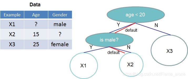
这里处理缺失值使用的方法是训练出默认的分支是左子树还是右子树。

具体的算法实现如下：

$\begin{array} { l } \text {Input: } I , \text { instance set of current node } \\ \text {Input: } I _ { k } = \left\{ i \in I | x _ { i k } \neq \text { missing } \right\} \\ \text {Input: } d , \text { feature dimension } \\ \text {Also applies to the approximate setting, only collect statistics of non-missing entries into buckets } \\ \operatorname { gain } \leftarrow 0 \\ G \leftarrow \sum _ { i \in I } , g _ { i } , H \leftarrow \sum _ { i \in I } h _ { i } \\ \text {for } k = 1 \text { to } m \text { do } \\ \qquad \begin{array} { l } \text {// enumerate missing value goto right } \\ G _ { L } \leftarrow 0 , H _ { L } \leftarrow 0 \\ \text {for } j \text { in sorted } \left( I _ { k } , \text { ascent order } b y \mathbf { x } _ { j k } \right) \text { do } \\ \qquad G _ { L } \leftarrow G _ { L } + g _ { j } , H _ { L } \leftarrow H _ { L } + h _ { j } \\ \qquad G _ { R } \leftarrow G - G _ { L } , H _ { R } \leftarrow H - H _ { L } \\ \qquad \text {score } \leftarrow \max \left( \text { score } , \frac { G _ { L } ^ { 2 } } { H _ { L } + \lambda } + \frac { G _ { R } ^ { 2 } } { H _ { R } + \lambda } - \frac { G ^ { 2 } } { H + \lambda } \right) \\ \text {end } \\ \text {// enumerate missing value goto left } \\ G _ { R } \leftarrow 0 , H _ { R } \leftarrow 0 \\ \text {for } j \text { in sorted } \left( I _ { k } , \text { descent order } b y \mathbf { x } _ { j k } \right) \text { do } \\ \qquad G _ { R } \leftarrow G _ { R } + g _ { j } , H _ { R } \leftarrow H _ { R } + h _ { j } \\ \qquad G _ { L } \leftarrow G - G _ { R } , H _ { L } \leftarrow H - H _ { R } \\ \qquad \text {score } \leftarrow \max \left( \text { score } , \frac { G _ { L } ^ { 2 } } { H _ { L } + \lambda } + \frac { G _ { R } ^ { 2 } } { H _ { R } + \lambda } - \frac { G ^ { 2 } } { H + \lambda } \right) \\\text {end } \\ \text {Output split and default directions with max gain } \end{array} \end{array}$

基本的实现方式就是将不缺失该特征的样本，只向左子树样本集（或右子树样本集）添加，那么缺失该特征的样本将会直接分配在右子树样本集（或左子树样本集），并且穷举全部可能，这样便可以求出哪种默认操作（向左子树样本集还是右子树样本集添加）更好一些。

并行学习（Column Block for Parallel Learning）

树学习最耗时的部分是将数据排序。为了降低排序的成本，建议将数据存储在内存单元中，作者将其称为块（block）。每个块中的数据以压缩列（compressed column，CSC）格式存储，每列按相应的特征值排序。这个输入数据布局只需要在训练之前计算一次，并且可以在以后的迭代中重用。下图便是这种块实现和使用流程：

可见其在存储特征值的同时也将特征值指向的梯度（或二阶梯度）值进行了存储。这使得并行计算全部特征的损失函数值成为了可能。

缓存优化（Cache-aware Access）

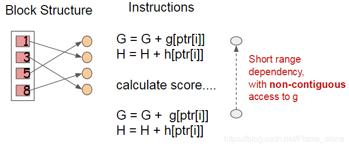
使用Block结构的一个缺点是取梯度（或二阶梯度）值的时候，是通过索引来获取的，而这些梯度的获取顺序是按照特征的大小顺序的。虽然时间复杂度为 $O(1)$，但这将导致梯度的获取是非连续的内存访问，可能使得CPU缓存命中率低，从而影响算法效率。

因此，在精准贪心算法中, 提出使用缓存预取算法。具体来说，对每个线程分配一个连续的缓存，按照特征值的排列顺序，以小批量的方式依次读取梯度信息并存入该连续缓存中，这样只需要一次非连续读取。该方式在训练样本数大的时候可以有效减小运算开销。

参考论文：XGBoost: A Scalable Tree Boosting System