Comparing Signals with Different Sampling Rates
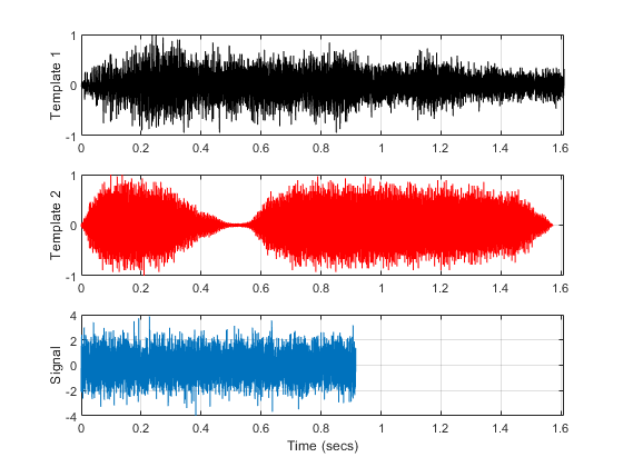
The first and the second subplot show the template signals from the database. The third subplot shows the signal which we want to search for in our database. Just by looking at the time series, the signal does not seem to match to any of the two templates. A closer inspection reveals that the signals actually have different lengths and sampling rates.
4096 4096 8192
Different lengths prevent you from calculating the difference between two signals but this can easily be remedied by extracting the common part of signals. Furthermore, it is not always necessary to equalize lengths. Cross-correlation can be performed between signals with different lengths, but it is essential to ensure that they have identical sampling rates.
Finding a Signal in a Measurement
We can now cross-correlate signal S to templates T1 and T2 with the xcorr function to determine if there is a match.
[C1,lag1] = xcorr(T1,S);
[C2,lag2] = xcorr(T2,S);
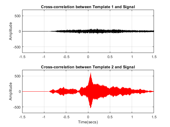
The first subplot indicates that the signal and template 1 are less correlated while the high peak in the second subplot indicates that signal is present in the second template.
[~,I] = max(abs(C2));
SampleDiff = lag2(I)
SampleDiff = 499
timeDiff = SampleDiff/Fs
timeDiff = 0.0609
The peak of the cross correlation implies that the signal is present in template T2 starting after 61 ms. In other words, signal T2 leads signal S by 499 samples as indicated by SampleDiff. This information can be used to align the signals.

Measuring Delay Between Signals and Aligning Them
Assume you have 3 sensors working at same sampling rates and they are measuring signals caused by the same event.
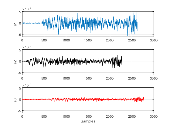
We can also use the finddelay function to find the delay between two signals.
t21 = finddelay(s1,s2)
t21 = -350
t31 = finddelay(s1,s3)
t31 = 150
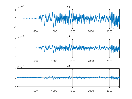
t21 indicates that s2 lags s1 by 350 samples, and t31 indicates that s3 leads s1 by 150 samples. This information can now used to align the 3 signals by time shifting the signals. We can also use the alignsignals function directly to align the signals which aligns two signals by delaying the earliest signal.
s1 = alignsignals(s1,s3);
s2 = alignsignals(s2,s3);
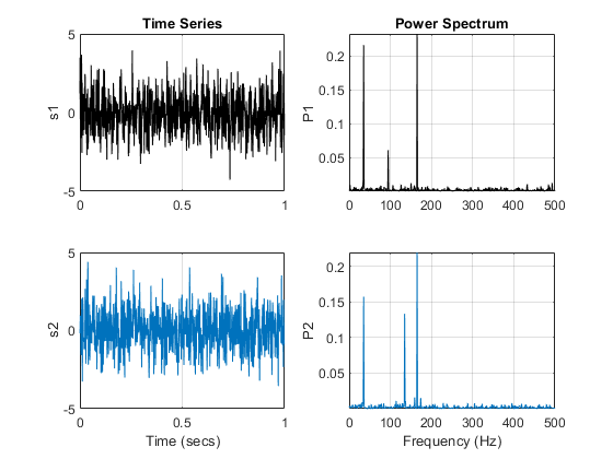
Comparing the Frequency Content of Signals
A power spectrum displays the power present in each frequency. Spectral coherence identifies frequency-domain correlation between signals. Coherence values tending towards 0 indicate that the corresponding frequency components are uncorrelated while values tending towards 1 indicate that the corresponding frequency components are correlated. Consider two signals and their respective power spectra.
The mscohere function calculates the spectral coherence between the two signals. It confirms that sig1 and sig2 have two correlated components around 35 Hz and 165 Hz. In frequencies where spectral coherence is high, the relative phase between the correlated components can be estimated with the cross-spectrum phase.
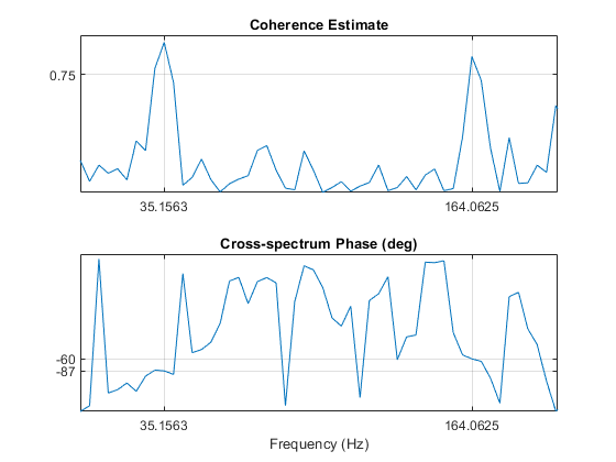
The phase lag between the 35 Hz components is close to -90 degrees, and the phase lag between the 165 Hz components is close to -60 degrees.
Finding Periodicities in a Signal
Consider a set of temperature measurements in an office building during the winter season. Measurements were taken every 30 minutes for about 16.5 weeks.
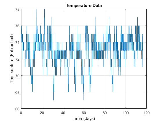
With the temperatures in the low 70s, you need to remove the mean to analyze small fluctuations in the signal. The xcov function removes the mean of the signal before computing the cross-correlation. It returns the cross-covariance.
maxlags = numel(temp)*0.5;
[xc,lag] = xcov(temp,maxlags);

[~,df] = findpeaks(xc,'MinPeakDistance',5*2*24);
[~,mf] = findpeaks(xc);
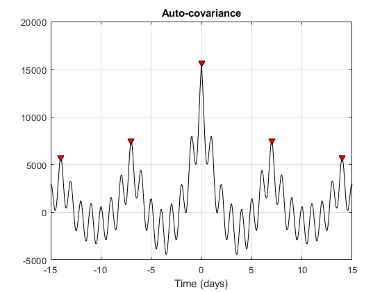
Observe dominant and minor fluctuations in the auto-covariance. Dominant and minor peaks appear equidistant. To verify if they are, compute and plot the difference between the locations of subsequent peaks.
cycle1 = diff(df)/(2*24);
cycle2 = diff(mf)/(2*24);

mean(cycle1)
ans = 7
mean(cycle2)
ans = 1.0000
The minor peaks indicate 7 cycles/week and the dominant peaks indicate 1 cycle per week. This makes sense given that the data comes from a temperature-controlled building on a 7 day calendar. The first 7-day cycle indicates that there is a weekly cyclic behavior of the building temperature where temperatures lower during the weekends and go back to normal during the week days. The 1-day cycle behavior indicates that there is also a daily cyclic behavior - temperatures lower during the night and increase during the day.
Reference
1. MathWorks