import numpy as np
import pandas as pd
import statsmodels.api as sm
import matplotlib.pyplot as plt
import seaborn as sns
sns.set()
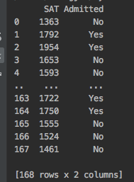
raw_data = pd.read_csv('2.01. Admittance.csv')
print(raw_data)
print("*****")
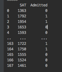
# like dummies, we must convert Yes/No to 1s and 0s
data = raw_data.copy()
data['Admitted'] = data['Admitted'].map({'Yes':1, 'No':0})
print(data)
print("*****")
# Declare the dependent and the independent variables
y = data['Admitted']
x1 = data['SAT']
plt.scatter(x1,y,color='C0')
plt.xlabel('SAT', fontsize=20)
plt.ylabel('Admitted', fontsize = 20)
plt.show() #This is pretty strange scatter plot
print("*****")
# Plot with a regression line
x = sm.add_constant(x1)
reg_lin = sm.OLS(y,x)
results_lin = reg_lin.fit()
plt.scatter(x1,y,color='C0')
y_hat = x1*results_lin.params[1] + results_lin.params[0]
plt.plot(x1, y_hat, lw=2.5, color='C8')
plt.xlabel('SAT', fontsize=20)
plt.ylabel('Admitted', fontsize=20)
plt.show() # This regression doesn't even know that our values are bounded between 0 and 1
print("*****")
# Plot with logistic regression curve
reg_log = sm.Logit(y,x)
results_log = reg_log.fit()
def f(x, b0, b1):
return np.array(np.exp(b0+x*b1) / (1 + np.exp(b0+x*b1)))
f_sorted = np.sort(f(x1, results_log.params[0], results_log.params[1]))
x_sorted = np.sort(np.array(x1))
plt.scatter(x1, y, color='C0')
plt.xlabel('SAT', fontsize = 20)
plt.ylabel('Admitted', fontsize = 20)
plt.plot(x_sorted, f_sorted, color='C8')
# Called Logistic Regression Curve
plt.show() # When the SAT score is relatively LOW, the probability of getting admitted is 0
print("*****")
"""
1. The Logistic regression predicts the probability of an event occuring
2. The logistic function has an S shape and is bounded by 0 and 1
"""
# Regression
x = sm.add_constant(x1)
reg_Log = sm.Logit(y,x)
# Stat's model as most modern libraries use the machine learning algorithm to fit the regression
# The function value shows the value of the objective function.
# There is always the possibility that after a certain number of iterations the model won't learn the relationship
# Therefore, it cannot optimize the optimization function in stat's models.
results_Log = reg_Log.fit()
print(results_Log.summary())
"""
1. Maximum likelihood estimation (MLE)
2. Likelihood function: A function which estimates how likely it is that the model at hand describes the real underlying relationship of
the variables
3. The bigger the likelihood function, the higher the probability that our model is correct!
4. MLE tries to maximize the likelihood function
5. The computer is going through different values, until it finds a model, for which the likelihood is the highest. When it can no longer
improve it, it will just stop the optimization.
6. Log-likelihood: it is time and tell you that it is much more convenient to take the log-likelihood we had when performing MLV.
Because of this convenience the log likelihood is the more popular metric. The value of the log-likelihood is almost but not always negative.
And the bigger it is the better.
7. LL-Null is the log-likelihood of a model which has no independent variables
8.
"""
print("*******")
x0 = np.ones(168)
reg_Log = sm.Logit(y, x0)
results_Log = reg_Log.fit()
print(results_Log.summary())
"""
1. LLR is the Log Likelihood ratio
It measures if our model is statistically different from LL-null. a.k.a, a useless model
2. Pseudo R-squ: it is somewhere between 0.2 and 0.4. Moreover this measure is mostly useful for comparing variations of the same model. Different model
will have completely different and incomparable Pseudo R-squares.
"""
print("*******")
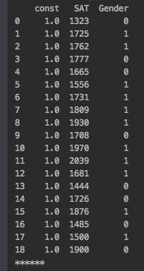
Raw_data = pd.read_csv('2.02. Binary predictors.csv')
Data = Raw_data.copy()
Data['Admitted'] = Data['Admitted'].map({'Yes':1, 'No':0})
Data['Gender'] = Data['Gender'].map({'Female':1, 'Male':0})
print(Data)
print("*******")
# Declare the dependent and the independent variables
Y = Data['Admitted']
X1 = Data['Gender']
# Regression
X = sm.add_constant(X1)
Reg = sm.Logit(Y,X)
Results_Log = Reg.fit()
Results_Log.summary()
print(Results_Log.summary())
print("*******")
# Accuracy
np.set_printoptions(formatter={'float': lambda x: "{0:0.2f}".format(x)})
print(Results_Log.predict()) # Predicted values by the model
print(np.array(data['Admitted'])) # Actual values
print("******")
print(Results_Log.pred_table())
print("******")
cm_df = pd.DataFrame(Results_Log.pred_table())
cm_df.columns = ['Predicted 0', 'Predicted 1']
cm_df = cm_df.rename(index={0: 'Actual 0', 1: 'Actual 1'})
print(cm_df) # Confusion matrix. It shows how confused our model is
print("******")
cm = np.array(cm_df)
accuracy_train = (cm[0,0] + cm[1,1]) / cm.sum()
print(accuracy_train)
"""
1. Overfitting: Our training has focused on the particular training set so much, it has "missed the point"
The models is so super good at modeling the training data that they "miss the point"
Captures all the noise, thus "miss the point"
High train accuracy
Fix: split the initial dataset into two - training and test
Create the regression on the training data after we have the coefficients. We test the model on the test data by creating a confusion matrix and assessing the accuracy.
The whole point is that the mode has never seen the test data set
2. Underfitting: The model has not captured the underlying logic of the data
Doesn't capture any logic
Low train accuracy
3. A good model captures the underlying logic of the dataset.
High train accuracy
"""
# Testing the model and assessing its accuracy
test = pd.read_csv('2.03. Test dataset.csv')
test['Admitted'] = test['Admitted'].map({'Yes':1, 'No':0})
test['Gender'] = test['Gender'].map({'Female':1, 'Male':0})
# Will use our model to make predictions based on the test data
# Will compare those with the actual outcome
# Calculate the accuracy
# Create a confusion matrix
test_actual = test['Admitted']
test_data = test.drop(['Admitted'], axis=1)
test_data = sm.add_constant(test_data)
print(test_data)
print("******")
def confusion_matrix(data, actual_values, model):
"""
Data: data frame or array
It is a data frame formatted in the same way as your input data (without the actual values)
Actual_values: data frame or array
These are the actual values from the test_data
In the case of a logistic regression, it should be a single column with 0s and 1s
"""
pred_values = model.predict(data) # Predict the values using the Logit model
bins = np.array([0,0.5,1]) # Specify the bins
# Create a histogram where if values are between 0 and 0.5 tell will be considered 0
# if they are between 0.5 and 1, they will be considered 1
cm = np.histogram2d(actual_values, pred_values, bins=bins)[0]
# Calculate the accuracy
accuracy = (cm[0,0] + cm[1,1]) / cm.sum()
# Return the confusion matrix and the accuracy
return cm, accuracy
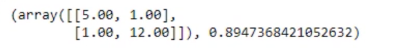
cm = confusion_matrix(test_data, test_actual, results_Log)
print(cm)