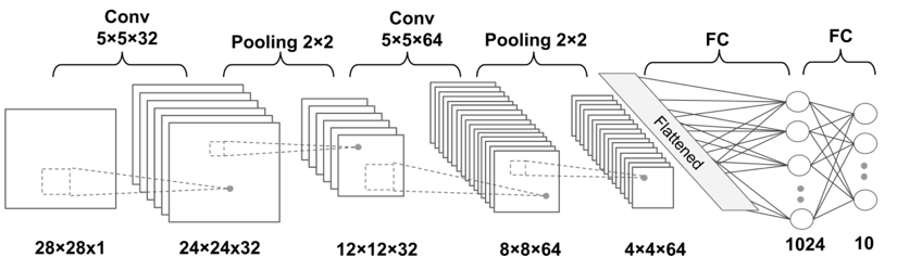
我们这次搭建的神经网络如下图所示:
它的输入是一个像素值为28*28的灰度图,然后输入的数据先经过一个卷积层,卷积核的大小是5*5*32,得到32个feature map,之后经过池化层,这里我们选择了最大池化,得到12*12*32的数据,此时再经过一个卷积层,卷积核为5*5*64,得到的结果再一次经过池化,得到的数据为4*4*64,最后通过一个全连接层,得到最终的结果。
1.下载和准备数据
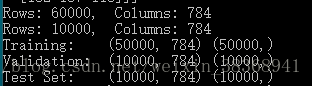
在这一部分我们完成对数据集的准备,这里我们选择最常见的书写数字图像集——MNIST,我们使用load_mnist函数来读取MNIST手写数字库,同时输出训练集、验证集、测试集的数量。
代码如下:
def
load_mnist(
path,
kind=
'train'):
"""Load MNIST data from `path`"""
labels_path = os.path.join(path,
'
%s
-labels-idx1-ubyte'
% kind)
images_path = os.path.join(path,
'
%s
-images-idx3-ubyte'
% kind)
with
open(labels_path,
'rb')
as lbpath:
magic, n = struct.unpack(
'>II',
lbpath.read(
8))
labels = np.fromfile(lbpath,
dtype=np.uint8)
with
open(images_path,
'rb')
as imgpath:
magic, num, rows, cols = struct.unpack(
">IIII",
imgpath.read(
16))
images = np.fromfile(imgpath,
dtype=np.uint8).reshape(
len(labels),
784)
return images, labels
X_data, y_data = load_mnist(
'./',
kind=
'train')
print(
'Rows:
%d
, Columns:
%d
' % (X_data.shape[
0], X_data.shape[
1]))
X_test, y_test = load_mnist(
'./',
kind=
't10k')
print(
'Rows:
%d
, Columns:
%d
' % (X_test.shape[
0], X_test.shape[
1]))
X_train, y_train = X_data[:
50000,:], y_data[:
50000]
X_valid, y_valid = X_data[
50000:,:], y_data[
50000:]
print(
'Training: ', X_train.shape, y_train.shape)
print(
'Validation: ', X_valid.shape, y_valid.shape)
print(
'Test Set: ', X_test.shape, y_test.shape)
输出结果如下:
2.生成模型前的准备工作
完成数据下载之后,此时我们需要从输入的数据中抽取股东size的batch,于是我们定义了batch生成函数。它返回一个数字+标签的元组。
代码如下:
def
batch_generator(
X,
y,
batch_size=
64,
shuffle=
False,
random_seed=
None):
idx = np.arange(y.shape[
0])
if shuffle:
rng = np.random.RandomState(random_seed)
rng.shuffle(idx)
X = X[idx]
y = y[idx]
for i
in
range(
0, X.shape[
0], batch_size):
yield (X[i:i+batch_size, :], y[i:i+batch_size])
接下来为了使得数据有更好的表现、更快的收敛,我们需要对数据进行归一下操作。我们计算每个feature的平均值和标准差,完成归一化操作。
代码如下:
mean_vals = np.mean(X_train,
axis=
0)
std_val = np.std(X_train)
X_train_centered = (X_train - mean_vals)/std_val
X_valid_centered = X_valid - mean_vals
X_test_centered = (X_test - mean_vals)/std_val
3.使用tensorflow的底层API搭建CNN网络
首先我们定义卷积层和全连接层,来简化搭建神经的过程。
首先是卷积层,这里我们定义了权重,误差,然后对他们进行初始化。这里的卷积操作使用tf.nn.conv2d函数,权重初始化使用Xavier,误差使用tf.zeros函数完成初始化,最后确定ReLU作为激活函数。
import tensorflow
as tf
import numpy
as np
## wrapper functions
def
conv_layer(
input_tensor,
name,
kernel_size,
n_output_channels,
padding_mode=
'SAME',
strides=(
1,
1,
1,
1)):
with tf.variable_scope(name):
## get n_input_channels:
## input tensor shape:
## [batch x width x height x channels_in]
input_shape = input_tensor.get_shape().as_list()
n_input_channels = input_shape[-
1]
weights_shape = (
list(kernel_size) +
[n_input_channels, n_output_channels])
weights = tf.get_variable(
name=
'_weights',
shape=weights_shape)
print(weights)
biases = tf.get_variable(
name=
'_biases',
initializer=tf.zeros(
shape=[n_output_channels]))
print(biases)
conv = tf.nn.conv2d(
input=input_tensor,
filter=weights,
strides=strides,
padding=padding_mode)
print(conv)
conv = tf.nn.bias_add(conv, biases,
name=
'net_pre-activation')
print(conv)
conv = tf.nn.relu(conv,
name=
'activation')
print(conv)
return conv
我们使用简单的输入来测试一下函数的功能:
g = tf.Graph()
with g.as_default():
x = tf.placeholder(tf.float32,
shape=[
None,
28,
28,
1])
conv_layer(x,
name=
'convtest',
kernel_size=(
3,
3),
n_output_channels=
32)
del g, x
得到结果如下,函数功能正常:

接下来我们定义全连接函数。同样地这里我们使用fc_layer来构建权重和误差,用conv_layer来初始化他们,接着然后使用tf.matmul函数完成生成矩阵。这个函数中有三个变量,分别为输入,该层的名称,用于确定范围、输出单元。
代码如下:
def
fc_layer(
input_tensor,
name,
n_output_units,
activation_fn=
None):
with tf.variable_scope(name):
input_shape = input_tensor.get_shape().as_list()[
1:]
n_input_units = np.prod(input_shape)
if
len(input_shape) >
1:
input_tensor = tf.reshape(input_tensor,
shape=(-
1, n_input_units))
weights_shape = [n_input_units, n_output_units]
weights = tf.get_variable(
name=
'_weights',
shape=weights_shape)
print(weights)
biases = tf.get_variable(
name=
'_biases',
initializer=tf.zeros(
shape=[n_output_units]))
print(biases)
layer = tf.matmul(input_tensor, weights)
print(layer)
layer = tf.nn.bias_add(layer, biases,
name=
'net_pre-activation')
print(layer)
if activation_fn
is
None:
return layer
layer = activation_fn(layer,
name=
'activation')
print(layer)
return layer
接着继续使用简单的输入验证函数功能。
g = tf.Graph()
with g.as_default():
x = tf.placeholder(tf.float32,
shape=[
None,
28,
28,
1])
fc_layer(x,
name=
'fctest',
n_output_units=
32,
activation_fn=tf.nn.relu)
del g, x
输出结果如下:

进行到这里,重头戏来了,我们要正式开始搭建CNN网络啦。。这里我们定义build_CNN 来管理搭建CNN模型的过程。
代码如下:
def
build_cnn():
## Placeholders for X and y:
tf_x = tf.placeholder(tf.float32,
shape=[
None,
784],
name=
'tf_x')
tf_y = tf.placeholder(tf.int32,
shape=[
None],
name=
'tf_y')
# reshape x to a 4D tensor:
# [batchsize, width, height, 1]
tf_x_image = tf.reshape(tf_x,
shape=[-
1,
28,
28,
1],
name=
'tf_x_reshaped')
## One-hot encoding:
tf_y_onehot = tf.one_hot(
indices=tf_y,
depth=
10,
dtype=tf.float32,
name=
'tf_y_onehot')
## 1st layer: Conv_1
print(
'
\n
Building 1st layer: ')
h1 = conv_layer(tf_x_image,
name=
'conv_1',
kernel_size=(
5,
5),
padding_mode=
'VALID',
n_output_channels=
32)
## MaxPooling
h1_pool = tf.nn.max_pool(h1,
ksize=[
1,
2,
2,
1],
strides=[
1,
2,
2,
1],
padding=
'SAME')
## 2n layer: Conv_2
print(
'
\n
Building 2nd layer: ')
h2 = conv_layer(h1_pool,
name=
'conv_2',
kernel_size=(
5,
5),
padding_mode=
'VALID',
n_output_channels=
64)
## MaxPooling
h2_pool = tf.nn.max_pool(h2,
ksize=[
1,
2,
2,
1],
strides=[
1,
2,
2,
1],
padding=
'SAME')
## 3rd layer: Fully Connected
print(
'
\n
Building 3rd layer:')
h3 = fc_layer(h2_pool,
name=
'fc_3',
n_output_units=
1024,
activation_fn=tf.nn.relu)
## Dropout
keep_prob = tf.placeholder(tf.float32,
name=
'fc_keep_prob')
h3_drop = tf.nn.dropout(h3,
keep_prob=keep_prob,
name=
'dropout_layer')
## 4th layer: Fully Connected (linear activation)
print(
'
\n
Building 4th layer:')
h4 = fc_layer(h3_drop,
name=
'fc_4',
n_output_units=
10,
activation_fn=
None)
## Prediction
predictions = {
'probabilities' : tf.nn.softmax(h4,
name=
'probabilities'),
'labels' : tf.cast(tf.argmax(h4,
axis=
1), tf.int32,
name=
'labels')
}
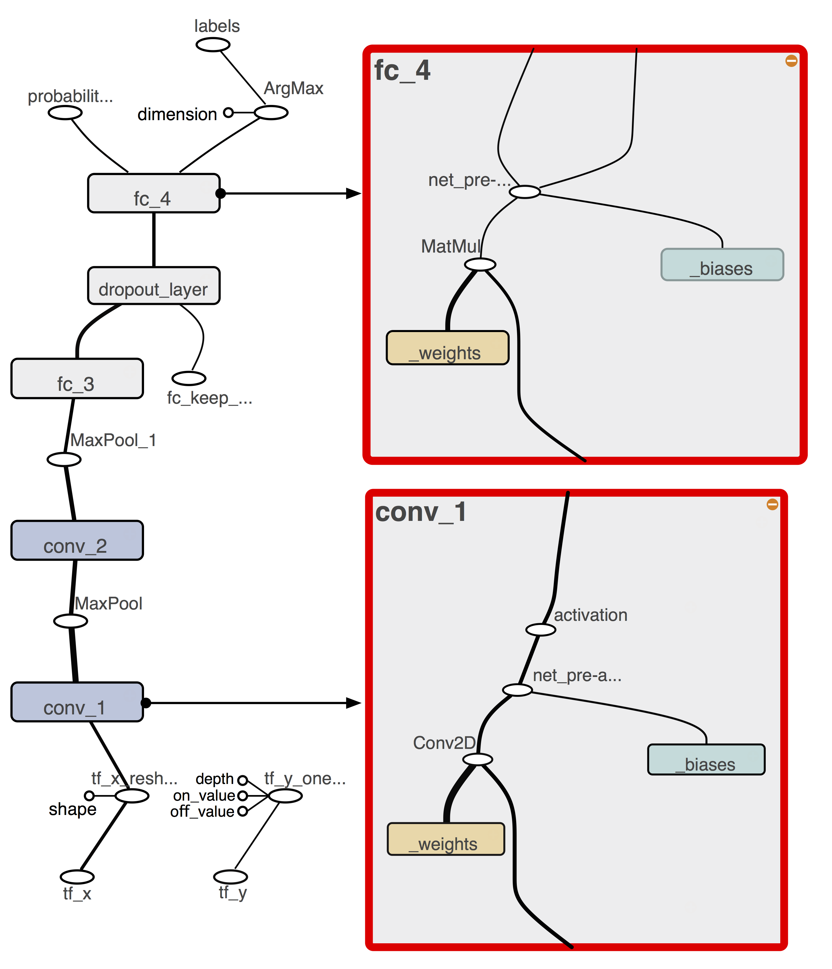
## Visualize the graph with TensorBoard:
## Loss Function and Optimization
cross_entropy_loss = tf.reduce_mean(
tf.nn.softmax_cross_entropy_with_logits(
logits=h4,
labels=tf_y_onehot),
name=
'cross_entropy_loss')
## Optimizer:
optimizer = tf.train.AdamOptimizer(learning_rate)
optimizer = optimizer.minimize(cross_entropy_loss,
name=
'train_op')
## Computing the prediction accuracy
correct_predictions = tf.equal(
predictions[
'labels'],
tf_y,
name=
'correct_preds')
accuracy = tf.reduce_mean(
tf.cast(correct_predictions, tf.float32),
name=
'accuracy')
这里得到的tensorboard结果如下:
接下来我们将定义四个其他函数:保存和加载函数以保存加载训练模型的检查点,训练模型使用training_set,预测函数来得到测试数据标签或可能性。
代码如下:
def
save(
saver,
sess,
epoch,
path=
'./model/'):
if
not os.path.isdir(path):
os.makedirs(path)
print(
'Saving model in
%s
' % path)
saver.save(sess, os.path.join(path,
'cnn-model.ckpt'),
global_step=epoch)
def
load(
saver,
sess,
path,
epoch):
print(
'Loading model from
%s
' % path)
saver.restore(sess, os.path.join(
path,
'cnn-model.ckpt-
%d
' % epoch))
def
train(
sess,
training_set,
validation_set=
None,
initialize=
True,
epochs=
20,
shuffle=
True,
dropout=
0.5,
random_seed=
None):
X_data = np.array(training_set[
0])
y_data = np.array(training_set[
1])
training_loss = []
## initialize variables
if initialize:
sess.run(tf.global_variables_initializer())
np.random.seed(random_seed)
# for shuflling in batch_generator
for epoch
in
range(
1, epochs+
1):
batch_gen = batch_generator(
X_data, y_data,
shuffle=shuffle)
avg_loss =
0.0
for i,(batch_x,batch_y)
in
enumerate(batch_gen):
feed = {
'tf_x:0': batch_x,
'tf_y:0': batch_y,
'fc_keep_prob:0': dropout}
loss, _ = sess.run(
[
'cross_entropy_loss:0',
'train_op'],
feed_dict=feed)
avg_loss += loss
training_loss.append(avg_loss / (i+
1))
print(
'Epoch
%02d
Training Avg. Loss:
%7.3f
' % (
epoch, avg_loss),
end=
' ')
if validation_set
is
not
None:
feed = {
'tf_x:0': validation_set[
0],
'tf_y:0': validation_set[
1],
'fc_keep_prob:0':
1.0}
valid_acc = sess.run(
'accuracy:0',
feed_dict=feed)
print(
' Validation Acc:
%7.3f
' % valid_acc)
else:
print()
def
predict(
sess,
X_test,
return_proba=
False):
feed = {
'tf_x:0': X_test,
'fc_keep_prob:0':
1.0}
if return_proba:
return sess.run(
'probabilities:0',
feed_dict=feed)
else:
return sess.run(
'labels:0',
feed_dict=feed)
现在我们可以创建一个tensorflow图形对象,生成图形的随机种子,并在该图中建立CNN模型
import tensorflow
as tf
import numpy
as np
## Define hyperparameters
learning_rate =
1e-4
random_seed =
123
np.random.seed(random_seed)
## create a graph
g = tf.Graph()
with g.as_default():
tf.set_random_seed(random_seed)
## build the graph
build_cnn()
## saver:
saver = tf.train.Saver()
接下来我们训练CNN模型,实现过程中首先创建Tensorflow session来发布表格,然后使用train函数
在第一次创建网络时,需要初始化各个变量。
代码如下:
with tf.Session(
graph=g)
as sess:
train(sess,
training_set=(X_train_centered, y_train),
validation_set=(X_valid_centered, y_valid),
initialize=
True,
random_seed=
123)
save(saver, sess,
epoch=
20)
得到结果如下:
在20个epochs完成后,我们保存之前训练的模型。实现过程中我们首先删除了graph g,新定义了g2
重组了训练模型,完成对测试集的预测。
### Calculate prediction accuracy
### on test set
### restoring the saved model
del g
## create a new graph
## and build the model
g2 = tf.Graph()
with g2.as_default():
tf.set_random_seed(random_seed)
## build the graph
build_cnn()
## saver:
saver = tf.train.Saver()
## create a new session
## and restore the model
with tf.Session(
graph=g2)
as sess:
load(saver, sess,
epoch=
20,
path=
'./model/')
preds = predict(sess, X_test_centered,
return_proba=
False)
print(
'Test Accuracy:
%.3f%%
' % (
100*
np.sum(preds == y_test)/
len(y_test)))
得到结果如下: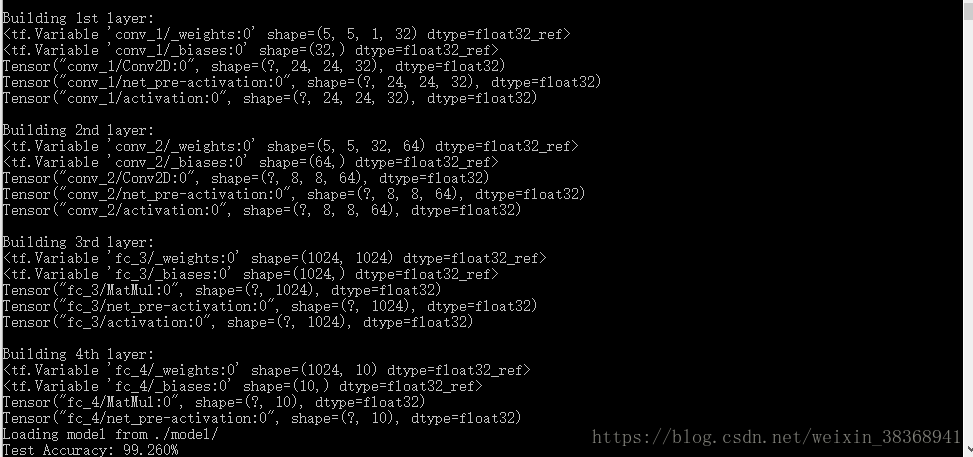
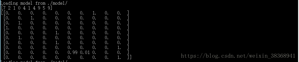
接着我们看一下前10个测试样本的预测情况。
## run the prediction on
## some test samples
np.set_printoptions(
precision=
2,
suppress=
True)
with tf.Session(
graph=g2)
as sess:
load(saver, sess,
epoch=
20,
path=
'./model/')
print(predict(sess, X_test_centered[:
10],
return_proba=
False))
print(predict(sess, X_test_centered[:
10],
return_proba=
True))
得到的结果如下:
接下来我们继续完成剩下的20个epoch,这次我们设置Initialize=False来跳过初始化操作。
## continue training for 20 more epochs
## without re-initializing :: initialize=False
## create a new session
## and restore the model
with tf.Session(
graph=g2)
as sess:
load(saver, sess,
epoch=
20,
path=
'./model/')
train(sess,
training_set=(X_train_centered, y_train),
validation_set=(X_valid_centered, y_valid),
initialize=
False,
epochs=
20,
random_seed=
123)
save(saver, sess,
epoch=
40,
path=
'./model/')
preds = predict(sess, X_test_centered,
return_proba=
False)
print(
'Test Accuracy:
%.3f%%
' % (
100*
np.sum(preds == y_test)/
len(y_test)))
得到的结果如下:
结果表明,20个附加时期的训练略有改善。在测试集上获得99.37%的预测精度。
